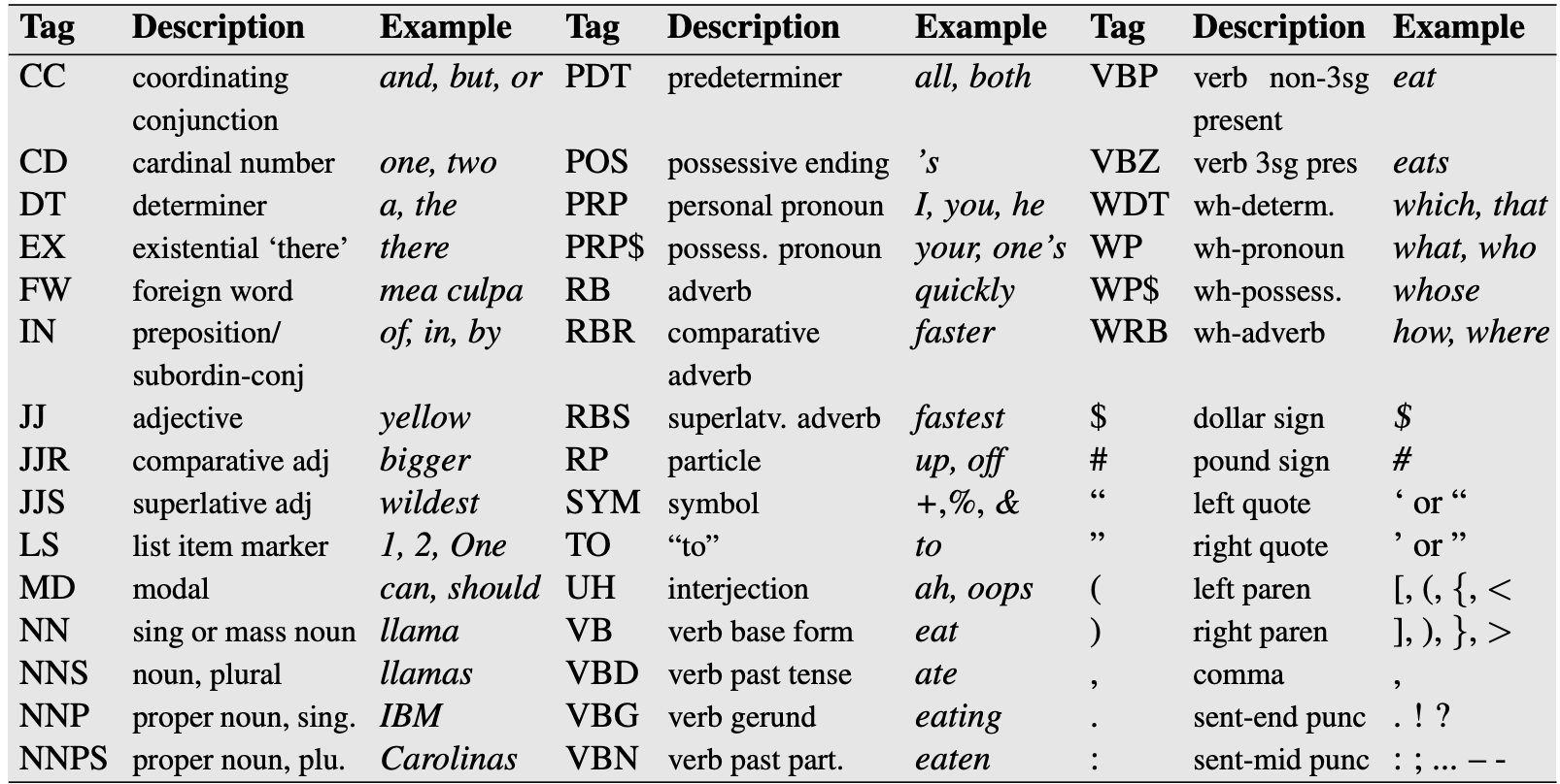
Hidden Markov Models for Parts-of-Speech Tagging

In Natural Language Processing (NLP), associating each word in a piece of text with a proper part of speech (POS) is known as POS tagging or POS annotation. POS tags are also known as word classes, morphological classes, or lexical tags.

Ambiguous words make POS tagging a nontrivial task. In each of the following sentences the word well belongs to a different part of speech.

• He did not feel very well. (adjective)

• She took it well, all things considered. (adverb)

• Well, this homework took me forever to complete. (interjection)

• The well is dry. (noun)

• Tears were beginning to well in their eyes. (verb)

Back in the days, the POS annotation was done manually. Assigning POS tags manually within modern multibillion-word corpora is unrealistic and automatic tagging is used instead.

Nowadays, manual annotation is typically used on a small portion of a text to create training data. After that, different techniques, such as transformation based tagging, deep learing models, and probabilistic tagging, can be used to develop an automated POS tagger.

• Transformation based approaches combine handcrafted rules (e.g., if an unknown word ends with the suffix “ing” and is preceded by a verb, label it as a verb) and automatically induced rules that are generated during the training.

• Deep learning tools, such as highly accurate Meta-BiLSTM, assign POS tags to words based on the discovered patterns during the training.

• Probabilistic tagging consists of a wide range of models. For example, it includes simple models that find the most frequently assigned tag for a specific word in the annotated training data and use this information to tag that word in the unannotated text. Hidden Markov Models also belong to probabilistic models for POS tagginng.

Hidden and observable states

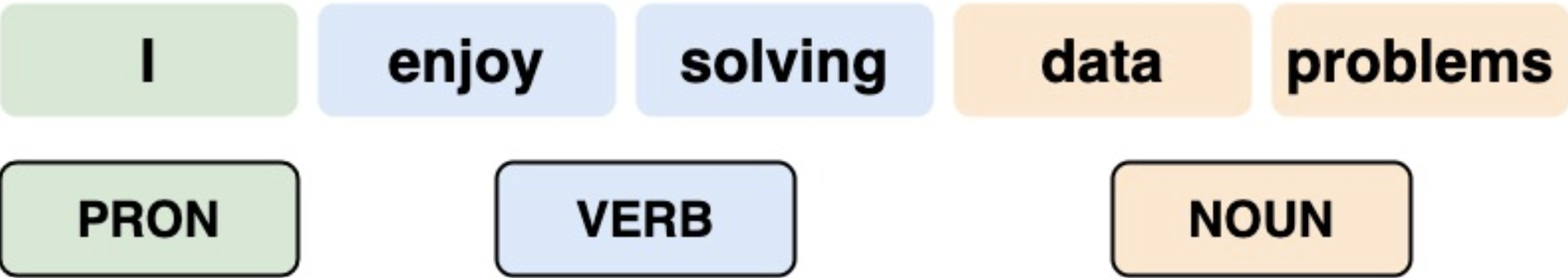
When we use HMMs for POS tagging, the tags serve as the hidden states and the words represent the observable states. If we distinquish only between nouns (\(NN\)), verbs
(\(VB\)), and other (\(O\)) tags, then \(NN\), \(VB\), and \(O\) represent the hidden states. The observable states can be going, to, walk, etc.

Calculating probabilities

How do we define the transition and emission probabilities for POS tagging?
We will introduce the computation of the probabilities based on the following toy corpus:

For simplicity we will distinquish only between nouns (\(NN\)), verbs (\(VB\)), and other (\(O\)) tags.

Transition probabilities

We assign blue background color to verbs, pink to nouns, and green to other parts of speech:

The number of times that a green tag is followed by a blue tag is 2. At the same time, the number of all tag pairs starting with a green tag is 3. Therefore, the transition probability from a green tag to a blue one is \(\frac{2}{3}\). In other words, \(P(VB|O) = \frac{2}{3}\) for this example.

More formally, the transition probabilities for an HMM are computed in two steps.
Step 1: Count the occurences of tag pairs

\[L(t_{i-1}, t_i) \quad \forall i \in \{1,\dots, N\}.\]

Here, \(N\) is the total number of POS tags.
That is, for each pair of tags \((t_{i-1}, t_i)\), we count how many times tag \(t_{i-1}\) is followed by tag \(t_i\).
Step 2: Calculate the conditional probabilities using the obtained counts

\[P(x_n = t_i|x_{n-1} = t_{i-1}) = \frac{L(t_{i-1}, t_i)}{\sum_{j=1}^{N} L\left(t_{i-1}, t_j\right)}.\]

That it, we normalize the number of times that tag \(t_{i-1}\) is followed by tag \(t_i\) by the total number of tag pairs that start with tag \(t_{i-1}\).

Question. Compute \(P(NN|O)\) for the toy corpus.

Answer. \(P(NN|O) = \frac{1}{3}.\)

Emission probabilities

To compute the emission probabilities we need to count the co-occurrences of a part of speech tag with a specific word. For example, the word “We” occurs 2 times in our corpus, tagged with a green tag for \(O\) for other (i.e., not a verb nor a noun). In total, the green tag appears three times in this corpus. Thus, the probability that the hidden state \(O\) emits the word “We”, \(P(We|O)\), is \(\frac{2}{3}\).

Similarly to the transition probabilities, the emission probabilities for an HMM are also computed in two steps.
Step 1: Count the co-occurences of tags and words

\[L(t_{i}, w_k) \quad \forall i \in \{1,\dots, N\} \text{ and} \: \: \forall k \in \{1,\dots, K\}.\]

Here, \(K\) is the total number of words.
That is, for each tag-word pair \((t_{i}, w_k)\), we count how many times the word \(w_k\) is associated with the tag \(t_i\).
Step 2: Calculate the conditional probabilities using the obtained counts

\[P(o_n = w_k|x_n = t_{i}) = \frac{L(t_{i}, w_k)}{\sum_{j=1}^{K} L\left(t_{i}, w_j\right)}.\]

That is, to find the conditional probabilities we divide \(L(t_{i}, w_k)\) by the total number of words associated with the same tag.

Question. Find \(P(The|O)\) and \(P(algorithm|NN)\) for the toy corpus.

Answer. \(P(The|O) = \frac{1}{3}\) and \(P(algorithm|NN) = 1.\)

POS tagging with Viterbi algorithm

Let us illustrate the full process of POS tagging with HMMs on the next example.

Corpus

We will use the set of sentences below to define the model.

• Mary Jane can see Will.

• Today Spot will see Mary.

• Will Jane spot Mary?

• Mary will pat Spot.

Observed sequence

Our goal is to annotate the following sentence:

Will can spot Mary.

Hidden states

For this example, we will distinquish between four hidden states: noun (\(NN\)), modal verb
(\(MD\)), verb (\(VB\)), and other (\(O\)) POS tags.

Pre-processing

Before we can construct the HMM, we need to identify the beginning of each sentence by adding the start of sentence tag <s>. In addition, we replace capital letters by lower case letters. The punctuation stays intact.

• <s> mary jane can see will.

• <s> today spot will see mary.

• <s> will jane spot mary?

• <s> mary will pat spot.

Manual annotation

Since the training set is relatively small, we can assign the tags manually, using color coding. Nouns are shown in red color, modal verbs in cyan, non-modal verbs in blue, and all other tags in green.

• <s> mary jane can see will.

• <s> today spot will see mary.

• <s> will jane spot mary?

• <s> mary will pat spot.

Transition probabilities

The below table shows the number of occurences of different tag pairs. It includes <s> tag that is needed to define the initial probabilities.

2nd tag\1st tag	<s>	\(NN\)	\(MD\)	\(VB\)	\(O\)
\(NN\)	2	1	1	4	1
\(MD\)	1	3	0	0	0
\(VB\)	0	1	3	0	0
\(O\)	1	4	0	0	0
Total	4	9	4	4	1

Dividing the number of occurences of each tag pair \((t_{i-1},t_i)\) by the total number of tag pairs that starts with tag \(t_{i-1}\) yields the transition matrix and the initial probabilities.

\[\begin{split} A = \begin{bmatrix} 1/9 & 1/4 & 1 & 1\\ 1/3 & 0 & 0 & 0 \\ 1/9 & 3/4 & 0 & 0\\ 4/9 & 0 & 0 & 0 \end{bmatrix} \: \text{ and } \: \pi = \begin{bmatrix} 1/2 \\ 1/4 \\ 0 \\ 1/4 \end{bmatrix}. \end{split}\]

Emission probabilities

The following table shows that in the considered corpus two words, will and spot, are used as different parts of speech.

word\tag	\(NN\)	\(MD\)	\(VB\)	\(O\)
mary	4	0	0	0
jane	2	0	0	0
will	1	3	0	0
spot	2	0	1	0
can	0	1	0	0
see	0	0	2	0
pat	0	0	1	0
today	0	0	0	1
.	0	0	0	3
?	0	0	0	1
Total	9	4	4	5

Dividing the number of co-occurences of a POS tag with a certain word by the total number of times the tag is used in the corpus provides us with the emission matrix.

\[\begin{split}B = \begin{bmatrix} 4/9 & 0 & 0 & 0\\ 2/9 & 0 & 0 & 0\\ 1/9 & 3/4 & 0 & 0\\ 2/9 & 0 & 1/4 & 0\\ 0 & 1/4 & 0 & 0\\ 0 & 0 & 1/2 & 0\\ 0 & 0 & 1/4 & 0\\ 0 & 0 & 0 & 1/5\\ 0 & 0 & 0 & 3/5\\ 0 & 0 & 0 & 1/5\\ \end{bmatrix}.\end{split}\]

Together \(A, B\) and \(\pi\) define the HMM.

The Viterbi algorithm

To assign POS tags to a sentence, we are going to use the Python implementation of the Viterbi algorithm that we introduced earlier.

# HMM: transition matrix, emission matrix, and initial probabilities
A = np.array([[1/9,1/4,1,1],[1/3,0,0,0],[1/9,3/4,0,0],[4/9,0,0,0]])
B = np.array([[4/9,0,0,0],[2/9,0,0,0],[1/9,3/4,0,0],[2/9,0,1/4,0],
              [0,1/4,0,0],[0,0,1/2,0],[0,0,1/4,0],[0,0,0,1/5],
              [0,0,0,3/5],[0,0,0,1/5]])
Pi = np.array([[1/2],[1/4],[0],[1/4]])

# Observed sequence: "Will can spot Mary."
O = np.array([2,4,3,0,8])

Note: The observed sequence is encoded in the same way as the emission matrix. For example, mary corresponds with index 0, jane with 1, etc.

# Result
X, C, D = Viterbi(O,A,B,Pi)
print("Matrix C: \n", C)
print("Matrix D: \n", D)
print("Answer: \n", X)

Matrix C: 
 [[5.55555556e-02 0.00000000e+00 2.57201646e-04 3.85802469e-04
  0.00000000e+00]
 [1.87500000e-01 4.62962963e-03 0.00000000e+00 0.00000000e+00
  0.00000000e+00]
 [0.00000000e+00 0.00000000e+00 8.68055556e-04 0.00000000e+00
  0.00000000e+00]
 [0.00000000e+00 0.00000000e+00 0.00000000e+00 0.00000000e+00
  1.02880658e-04]]
Matrix D: 
 [[0 1 2 3 1]
 [0 1 1 1 1]
 [0 1 2 1 1]
 [0 1 1 1 1]]
Answer: 
 [1 2 3 1 4]

From the computation of the transition matrix, we know that

• 1 represents a noun,

• 2 represents a modal verb,

• 3 represents a non-modal verb,

• 4 represents other POS tags.

This implies that the answer that we obtained, \(\begin{bmatrix} 1 & 2 & 3 & 1 & 4 \end{bmatrix}\), corresponds with the following sequesnce of POS tags:
noun, modal verb, non-modal verb, noun, and other tag.
The model assigned all the POS tags correctly, because the observed sequence was Will can spot Mary.

What if we change the observed sequence? For example, we can replace it by

Today Jane can see Spot.

# Observed sequence: "Today Jane can see Spot."
O = np.array([7,1,4,5,3,8])

# Result
X, C, D = Viterbi(O,A,B,Pi)
print("Answer: \n", X)

Answer: 
 [4 1 2 3 1 4]

These tags are correct as well.

In general, HMM is a powerfull tool for POS tagging. However, it should be used with caution.

Smoothing

Consider one of the poems that was written by Ezra Pound:

In a Station of the Metro
The apparition of these faces in the crowd:
Petals on a wet, black bough.

Assume that the hiddent states are comprised of nouns, verbs, and other tags, then the tag-pair counts can be found in the below table.

2nd tag\1st tag	<s>	\(NN\)	\(VB\)	\(O\)
\(NN\)	1	0	0	6
\(VB\)	0	0	0	0
\(O\)	2	6	0	8
Total	3	6	0	14

The poem is verbless. For this reason, the total number of tag pairs that start with a verb is zero. Can we still compute the transition matrix?

Smoothing is a technique that can be used to avoid division by zero during the computation of the probabilities for an HMM. It can be achieved by adding a small number \(\varepsilon\), say 0.001, to the numerator and a multiple of that number for the denominator. More precisely, the smoothing of the transition probabilities can be achieved using the following formula

\[P(x_n=t_i|x_{n-1}=t_{i-1}) = \frac{L(t_{i-1}, t_i)+\varepsilon}{\sum_{j=1}^{N} L\left(t_{i-1}, t_j\right)+N\varepsilon}.\]

For emission probabilities, the formula with smoothing is given by

\[P(o_n=w_i|x_n=t_{i}) = \frac{L(t_{i}, w_k)+\varepsilon}{\sum_{j=1}^{K} L\left(t_{i}, w_j\right)+K\varepsilon}.\]

Adding \(N\varepsilon\) to the divisor allows the transition matrix to remain column stochastic. Similarly, the formula with smoothing for emission probabilities allows the emission matrix to stay column stochastic.

After smoothing the transition matrix for Pound’s poem is equal to

\[\begin{split}A = \begin{bmatrix} \frac{\varepsilon}{6+3\varepsilon} & \frac{1}{3} & \frac{6+\varepsilon}{14+3\varepsilon}\\[2pt] \frac{\varepsilon}{6+3\varepsilon} & \frac{1}{3} & \frac{\varepsilon}{14+3\varepsilon}\\[2pt] \frac{6+\varepsilon}{6+3\varepsilon} & \frac{1}{3} & \frac{8+\varepsilon}{14+3\varepsilon} \end{bmatrix},\end{split}\]

where \(\varepsilon\) can be any small number.

As can be seen from the above matrix, smoothing also reduces the sparsity of the matrix. This is another great feature of smoothing, because sparse matrices impair the performance of HMMs.

For example, without smoothing the transition probability from a noun to verb would be zero. Zero-probabilities would prevent the Viterbi algorithm from finding the most likely sequence of POS tags, if the observed sequence would contain verbs.

Summary

1. HMMs belong to probabilistic models for POS tagging. When HMMs are used to assign tags to words, tags serve as hidden states and words as observable states.

2. To compute the transition probability from tag \(t_{i-1}\) to tag \(t_i\), we count the occurences of the tag pair and divide that obtained number by the total number of tag pairs that start with \(t_{i-1}.\)

3. To compute the emission probability from tag \(t_i\) to word \(w_k\), we count the co-occurences of \(t_i\) and \(w_k\) and divide the obtained number by the total number of words with tag \(t_i\).

4. Smoothing can be used to improve the performance of HMMs, when many transition or emission probabilities are equal to zero.