Introduction and Probability Review
Contents
Introduction and Probability Review#
Today we will talk about different views on probability: frequentist and Bayesian.
In addition, we will review the essentials of probability that we will need for later parts of this course. These are recaps of concepts you covered in DS 120.
Probability#
What is probability?
We all have a general sense of what is meant by probability.
However, when we look closely, we see that there are at least two different ways to interpret the notion of “the probability of an event.”
The Frequentist View#
The frequentist view of probability requires the definition of several concepts.
Experiment: a situation in which the outcomes occur randomly.
Example: Driving to work, a commuter passes through a sequence of three intersections with traffic lights. At each light she either stops \(s\) or continues \(c\).
Sample space: the set of all possible outcomes of the experiment.
Example: \(\{ccc, ccs, csc, css, scc, ssc, scs, sss\},\) where \(csc\), for example, denotes the outcome that the commuter continues through the first light, stops at the second light, and continues through the third light.
Event: a subset of the sample space.
Example: continuing through the first light (i.e., \(\{ccc, ccs, csc, css\}\)).
The frequentist view is summarized by this quote from the first pages of a probability textbook:
Suppose an experiment under consideration can be repeated any number of times, so that, in principle at least, we can produce a whole series of “independent trials under identical conditions” in each of which, depending on chance, a particular event \(A\) of interest either occurs or does not occur.
Let \(n\) be the total number of experiments in the whole series of trials, and let \(n(A)\) be the number of experiement in which \(A\) occurs. Then the ratio \(n(A)/n\) is called the relative frequency of the event \(A.\)
It turns out that the relative frequencies observed in different series of trials are virtually the same for large \(n,\) clustering about some constant \(P[A],\) which is called the probability of the event \(A.\)
Y. A. Rozanov. Probability Theory: A Concise Course. 1969.
This is called the frequentist intepretation of probability.
The key idea in the above definition is to be able to:
produce a whole series of “independent trials under identical conditions”
Which, when you think about it, is really a rather tricky notion.
Nevertheless, the frequentist view of probability is quite useful and we will often use it in this course.
You can think of it as treating each event as a sort of idealized coin-flip.
In other words, when we use the frequentist view, we will generally be thinking of a somewhat abstract situation where we assume that “independent trials under identical conditions” is a good description of the situation.
The Bayesian View#
To understand the Bayesian view of probability, consider the following situations:
On a visit to the doctor, we may ask, “What is the probability that I have disease X?”
Or, before digging a well, we may ask, “What is the probability that I will strike water?”
These questions are totally incompatible with the notion of “independent trials under identical conditions”!
Either I do, or do not, have disease X. Either I will, or will not, strike water.
Rather, it seems that we are really asking:
“How certain should I be that I have disease X?”
“How certain should I be that I will strike water?”
In this setting, we are using probability to encode a “degree of belief” or a “state of knowledge.”
This is called the Bayesian interpretation of probability.
This point of view often seems more intuitive than the frequentist point of view. However, encoding a certain belief using probability can be tricky too.
For instance, consider the following example from Tversky and Kahneman, who posed the following question:
‘’Linda is 31 years old, single, outspoken, and very bright. She majored in philosophy. As a student, she was deeply concerned with issues of discrimination and social justice, and also participated in anti-nuclear demonstrations. Which is more probable?
Linda is a bank teller.
Linda is a bank teller and is active in the feminist movement.’’
Many people choose the second answer, presumably because it seems more consistent with the description. It seems uncharacteristic if Linda is just a bank teller; it seems more likely if she is also a feminist.
But the second answer cannot be “more probable”, as the question asks. Suppose we find 1000 people who fit Linda’s description and 10 of them work as bank tellers. How many of them are also feminists? At most, all 10 of them are; in that case, the two options are equally probable. If fewer than 10 are, the second option is less probable. But there is no way the second option can be more probable.
Somewhat amazingly, it turns out that whichever way we think of probability (frequentist or Bayesian),
… the rules that we use for computing probabilities should be exactly the same.
This is a very deep and surprising thing.
In other words, it’s often really a “state of knowledge” that we are really talking about when we use probability models in this course.
A thing appears random only through the incompleteness of our knowledge.
Spinoza, Ethics, Part 1
In other words, we use probability as an abstraction that hides details we don’t want to deal with.
So it’s important to recognize that both frequentist and Bayesian views are valid and useful views of probability.
What is Probability (and Statistics) Good For?#
Probability is the logic of uncertainty. In other words, when you are uncertain about something you need probability to make a decision on a rational (logical) basis.
So you will not be surprised to know that the roots of probability were developed to analyze games of chance - gambling.
In the mid 1650s, the mathematician Blaise Pascal was considering a particular gambling game. A friend asked him how to divide the winnings if the game ended early (before one player had completely won).
Pascal started a correspondence with another mathematician, Pierre Fermat, exchanging letters and discussing what would be a fair way to divide the pot. They developed the idea of listing all the possible ways the game could have gone, and dividing the winnings according to the number of outcomes in which each player wins the game. This led to the classical frequentist notion of probability that we use today.
But it turns out that gambling is far from the only setting where we are uncertain about the facts. Most of science consists of settings where there is some uncertainty about the facts. In finance we are typically uncertain about the future. In physics we are typicaly uncertain about the value of a measurement. In political science we are uncertain about public opinion. The lists go on and on. Probability is a crucial tool in almost every area of human endeavor.
The actual science of logic is conversant at present only with things either certain, impossible, or entirely doubtful, none of which (fortunately) we have to reason on. Therefore the true logic for this world is the calculus of Probabilities, which takes account of the magnitude of the probability which is, or ought to be, in a reasonable man’s mind.
James Clerk Maxwell (1850)
Probability and Conditioning#
As we’ve said, whether we are thinking of probability in a frequentist or a Bayesian sense, the rules that we use for manipulating probabilities are the same.

To motivate our definitions of probability and conditioning, let’s consider the following scenario.
Suppose some dark night a policeman walks down a street, apparently deserted. Suddenly he hears a burglar alarm, looks across the street, and sees a jewelry store with a broken window. Then a gentleman wearing a mask comes crawling out through the broken window, carrying a bag which turns out to be full of expensive jewelry. The policeman does not hesitate at all in deciding that this gentleman is dishonest. By what reasoning process does he arrive at this conclusion?
(From Probability Theory, E.T. Jaynes)
Clearly, it is possible that the gentleman is not a thief. The question is, what calculational rules should the policeman use to assign a probability to the idea that the gentleman is a thief?
Probability theory is nothing but common sense reduced to calculation.
Laplace, 1819
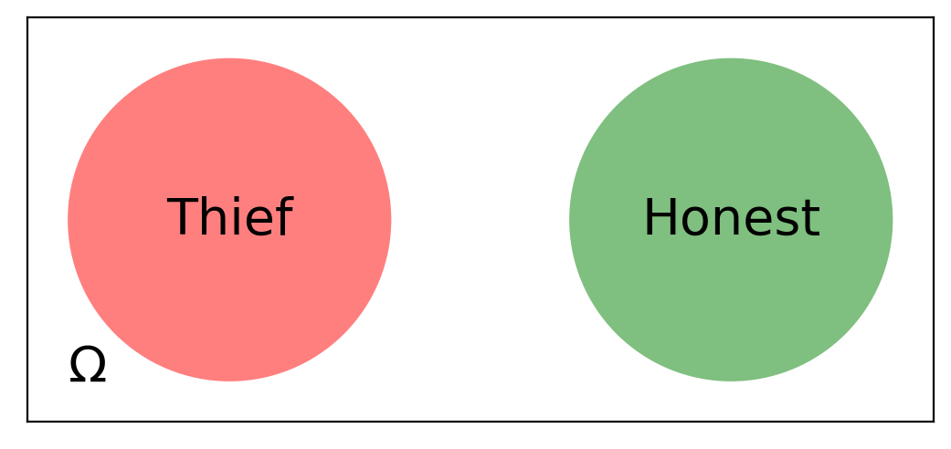
To start with, we’ll follow Pascal’s idea: write down all the possibilities. As we mentioned previously, they will form the sample space. We will denote it by \(\Omega\).
In this case \(\Omega = \{\text{thief}, \text{honest}\}\).
For each member of \(\Omega\) we will assign a number in the range \([0, 1]\) and call it the outcome’s probability.
We denote it with \(P\), so we might say \(P(\text{thief}) = 0.3.\)
(or whatever).
Here we are using the first axiom of probability.
Axiom 1: For each event \(E\) of the sample space \(\Omega\), \(P(E)\) satisfies
The second axiom tells us with probability 1, the outcome will be a point in the sample space.
Axiom 2:
The third axiom is concerned with disjoint or mutually exclusive events. These are events that do not co-occur.
Axiom 3: If \(E_1\) and \(E_2\) are disjoint than the probability that \(E_1\) or \(E_2\) occurs is equal to
Since a person cannot be a thief and honest at the same time, from Axiom 3 it follows that
Combining this with Axiom 2 we obtain
This is actually a well known fact about probabilities of the event \(E\) and its complement, \(\bar{E}.\)
Property A: \(P(\bar{E}) = 1 - P(E).\)
Since \(\overline{\Omega} = \emptyset\), this property tell us that the probability that there is no outcome at all is zero.
Property B: \(P(\emptyset) = 0.\)
Another important property in probability theory states that if the event \(E\) is contained in the event \(F\), then the probability of \(E\) is no greater than the probability of \(F\).
Property C: If \(E\) is contained in \(F\), then \(P(E) \leq P(F).\)
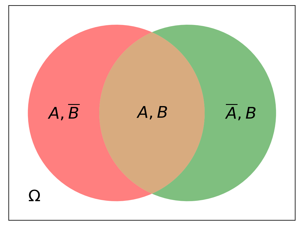
The last fundamental property tells us about the union of two events that can co-occur.
Property D: \(P(E \cup F) = P(E) + P(F) - P(E,F).\)
More than One Event#
When we start to consider multiple events, we need calculation rules for joint probabilities.
The event \(A,B\) means that both \(A\) and \(B\) are true.
So in our example we might be interested in \(P(\text{thief},\text{broken window})\).
In general, there is no simple rule for how to compute \(P(A, B)\).
It depends on how often the events co-occur.
Conditional Probability#
To follow the policeman’s reasoning, we need to use conditional probability. The conditional probability of \(A\) given \(B\), written
Is the probability of event \(A\) if we know that \(B\) is true.
For example, we are interested in:
Intuitively, we would expect that
And indeed the proper rule for computing this is:
We interpret this as dividing the probability that both events (\(A\) and \(B\)) occur by the probability that the conditioning event (\(B\)) occurs.
Note that we have to assume that \(P(B) > 0\). The condition does not make sense otherwise.
Finally, we’ll introduce the last calculational rule, which relates to independent events.
We say that events \(A\) and \(B\) are independent if the occurrence of one does not change the probability of the other.
That is, if \(A\) and \(B\) are independent, then
or, equivalently,
Intuitively, the knowledge that one event has occurred does not change our estimate of the probability of the other event.
For example, knowing the day of the week does not change our estimate of whether it will be raining or sunny.
Since \( P(A\,\vert\,B) = \frac{P(A, B)}{P(B)}\) and, for independent events \(A\) and \(B\), \(P(A\,\vert\,B) = P(A),\) we obtain $\( \frac{P(A, B)}{P(B)} = P(A). \)$
Hence,
when \(A\) and \(B\) are independent.
So, for example, let’s say that here in Boston about \(10\%\) of the days are rainy. What fraction of the days of the year are rainy Mondays?
What are the two events \(A\) and \(B\), and what are their probabilities?
\(P(A) = P(\text{day is rainy}) = 1/10\) and \(P(B) = P(\text{day is Monday}) = 1/7\)
What is the probabilty question we are asking?
\(P(A,B) = P(\text{day is rainy } and \text{ day is Monday})\)
Are the two events independent?
Yes!
Since we can assume independence, the answer is easy to compute:
So we expect about 365 / 70 = about 5 rainy Mondays per year.
Chain Rule#
Recall again the definition of conditional probability:
By rearranging terms, we can see that:
This is called the chain rule of conditional probabilities.
We can extend this pattern to as many random variables as we want. For example:
And this gives us the tools we need to write out a mathematical representation of the policeman’s logic!
The chain rule tells us that:
And we want to calculate:
Which we can get to by moving around some terms.
Law of Total Probability#
Another useful tool for computing probabilities is provided by the following law.
Let \(B_1\) and \(B_2\) form the complete sample space \(\Omega\) and be disjoint \(\left(B_1 \cap B_2 = \emptyset\right)\). Then for any event \(A\),
Bayes’ Rule#
Another direct consequence of the definition of conditional probability is Bayes’ Rule:
We won’t focus on it too much now, but we will use Bayes Rule a lot in this course, and we will discuss it more in upcoming lectures. The key insight, as we will see, is that we can use observations of \(B\) to update out belief in \(A\).
For now, think about how you might derive this rule from the rules we have learned so far.