Inference
Contents
Inference#
One of the most classic applications of frequentist stastistics is the comparison of two groups to see if there is a difference in their means.
How is this done in the Bayesian setting?
The Bayesian Approach#
A Bayesian alternative is to compute the posterior distribution of the difference between the groups.
Then we can use that distribution to answer whatever questions we are interested in, including:
the most likely size of the difference
a credible interval that’s likely to contain the true difference
the probability of superiority
the probability that the difference exceeds some threshold.
Example: Improving Reading Ability#
To demonstrate this process, we’ll solve a problem about evaluating the effect of an educational “treatment” compared to a control.

What’s the data?#
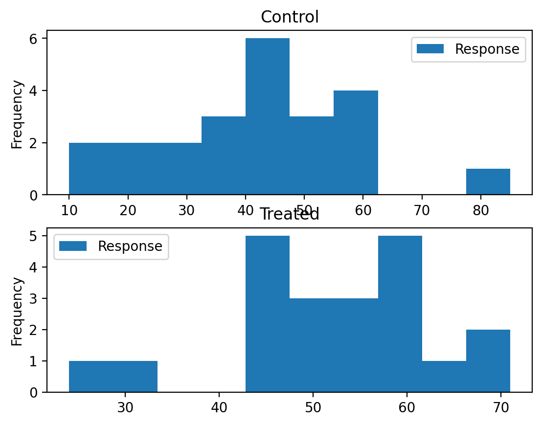
An educator conducted an experiment to test whether new directed reading activities in the classroom will help elementary school pupils improve some aspects of their reading ability. She arranged for a third grade class of 21 students to follow these activities for an 8-week period. A control classroom of 23 third graders followed the same curriculum without the activities. At the end of the 8 weeks, all students took a Degree of Reading Power (DRP) test, which measures the aspects of reading ability that the treatment is designed to improve.
df = pd.read_csv('images/drp_scores.csv')
df.head(3)
| Treatment | Response | |
|---|---|---|
| 0 | Treated | 24 |
| 1 | Treated | 43 |
| 2 | Treated | 58 |
Approaching the problem#
We’ll assume that for the entire population of students the distribution of scores is well modeled by a normal distribution with unknown mean and standard deviation.
We’ll use \(\mu\) and \(\sigma\) to denote these unknown parameters
And we’ll do a Bayesian update to estimate what they are.
To put it another way, we’ll use a Bayesian update to estimate paramaters for normal distributions that fit our data.
The Prior#
First we need a prior distribution for the parameters. Since there are two parameters, it will be a joint distribution.
We’ll assume that the prior distributions for \(\mu\) and \(\sigma\) are uniform:
from scipy.stats import randint

# uniform prior for mu
prior_mu  = pd.DataFrame(index = np.linspace(20, 80, num=101))
prior_mu ['probs'] = 1/101

#uniform prior for sigma
prior_sigma  = pd.DataFrame(index = np.linspace(5, 30, num=101))
prior_sigma ['probs'] = 1/101
And we’ll want to consider the joint distribtion of the two paramaters:
# multiplies prbabilities from two distributions
def make_joint(pmf1, pmf2):
    """Compute the outer product of two Pmfs."""
    X, Y = np.meshgrid(pmf1['probs'], pmf2['probs'])
    return pd.DataFrame(X * Y, columns=pmf1.index, index=pmf2.index)

prior = make_joint(prior_mu, prior_sigma)
The Likelihood#
We would like to know the probability of each score in the dataset for each hypothetical pair of values, \(\mu\) and \(\sigma\).
Put another way for each of our 101 possible \(\mu\)s and 101 possible \(\sigma\)s, we need to calculate the likelihood for each of our 44 students.
First let’s create a data object just to store all that information:
mu_mesh, sigma_mesh, data_mesh = np.meshgrid(prior.columns, prior.index, df.Response)
mu_mesh.shape
(101, 101, 44)
Then let’s calculate the probability of each score for each \(\mu\) and \(\sigma\):
from scipy.stats import norm

densities = norm(mu_mesh, sigma_mesh).pdf(data_mesh)
Finally, to get the actual likelihood of each \(\mu\) and \(\sigma\) we take the product across the data. We want likelihoods for the parameters for the control and treatment groups separately.
# control
likelihood_control = densities[:,:,df['Treatment']=="Control"].prod(axis=2)

# treated
likelihood_treated = densities[:,:,df['Treatment']=="Treated"].prod(axis=2)
likelihood_treated.shape
(101, 101)
The Update#
We’ll create posterier distriburions for control and treated the usual way:
# update with control likelihood
posterior_control = prior * likelihood_control
prob_data = posterior_control.to_numpy().sum()
posterior_control = posterior_control / prob_data

#update with treated likelihood
posterior_treated = prior * likelihood_treated
prob_data = posterior_treated.to_numpy().sum()
posterior_treated = posterior_treated / prob_data
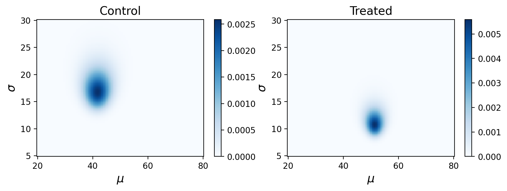
What are these posterior distributions actually conveying? It helps to visualize the probabilities:

Remember, this is showing the joint posterior probabilities for parameters that best describe our observed data.
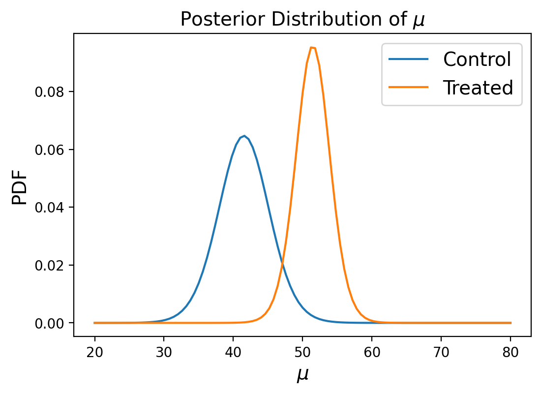
Posterior Marginal Distributions#
Just like in our previous example of using a joint distribution to model the heights of two individuals, we’ll look at posterior marginal distributions, except this time for each paramater rather than each measurement.
marginal_mean_control = posterior_control.sum(axis=0)
marginal_mean_treated = posterior_treated.sum(axis=0)
We can then compare the marginals of the two groups using the probability of superiority:
def prob_of_s(dist1, dist2):
    """Compute the probability of superiority."""
    total = 0
    for i1 in dist1.index:
        for i2 in dist2.index:
            if i1 > i2:
                total += dist1[i1] * dist2[i2]
    return total

prob_of_s(marginal_mean_treated, marginal_mean_control)
0.9804790251873254
Let’s compare that to a t-test, which would have been the frequentist approach given the small number of samples:
from scipy.stats import ttest_ind
ttest_ind(df.Response[df.Treatment=="Treated"],df.Response[df.Treatment=="Control"])
Ttest_indResult(statistic=2.266551599585943, pvalue=0.028629482832245753)
It’s good to see that these probabilities generally agree with each other!
Distribution of Differences#
Now let’s consider the difference in the two distributions:
def sub_dist(dist1, dist2):
    """Compute the distribution of a difference."""
    p_dist = pd.DataFrame(index=np.unique(np.subtract.outer(dist1.index, dist2.index).flatten()))
    # Ensure the 'probs' column is of float type
    p_dist['probs'] = 0.0

    for i1 in dist1.index:
        for i2 in dist2.index:
            q = i1 - i2
            p = dist1[i1] * dist2[i2]
            p_dist.loc[q, 'probs'] = p_dist.loc[q, 'probs'] + p

    return p_dist

pmf_diff = sub_dist(marginal_mean_treated, marginal_mean_control)
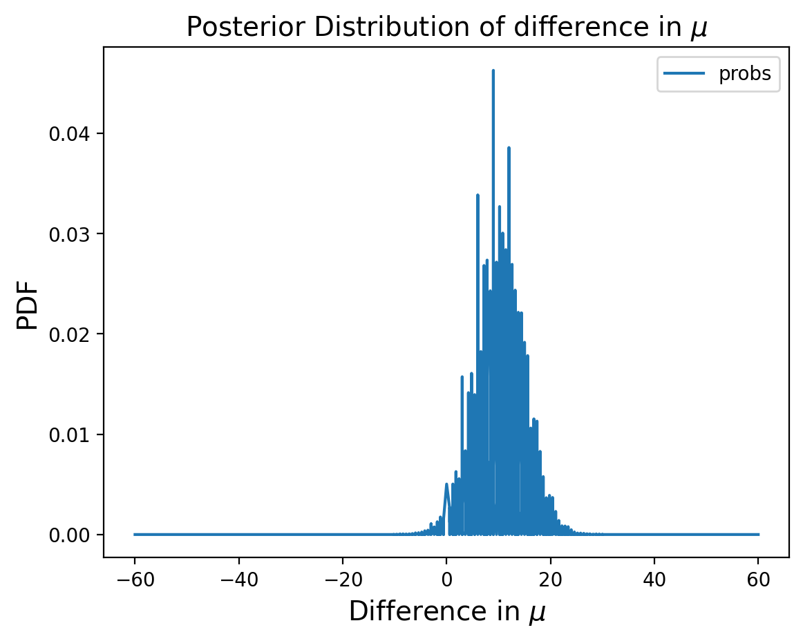
Let’s find the MMSE of the difference:
np.sum(pmf_diff.index * pmf_diff.probs)
9.954413088940848
And we can also calculate the probability that the difference is greater than some arbitrary value, lets say 5:
sum(pmf_diff.probs[pmf_diff.index>5])
0.8558784849055037
And the 90% credible interval:
[max(pmf_diff.index[np.cumsum(pmf_diff).probs < .05]), min(pmf_diff.index[np.cumsum(pmf_diff).probs > .95])]
[2.3999999999999915, 17.4]
So using the difference in posterior distributions of the means, we can learn everything we need to know about the difference in populations.
Empirical Bayes#
Recall that Empirical Bayes is statistical inference in which the prior probability distribution is estimated from the data.
For example for the train problem we reasoned that a train-operating company with 1000 locomotives is not just as likely as a company with only 1, so we switched from a uniform prior to a power law prior.
But we also noted that perhaps we could also directly use some data (e.g. a survey of train operators).
In some cases, we actually use the very same data we plan to use for our updates. This is in stark contrast with our standard procedue where the prior distribution is fixed before any data are observed (it’s always our first step before calculating any likelihoods).
Basically this means using data twice, once for the prior and once for the update. While that might seem problematic (and some data scientists think it is) its a commomly used strategy to construct priors.
For example, lets use the mean and standard deviation of the test scores for the prior distribution of \(\mu\) in the control/treatment data we’ve been using, and from there just run all the same code as before:
# empirical Bayes prior for mu
prior_mu  = pd.DataFrame(index = np.linspace(20, 80, num=101))
prior_mu ['probs'] = norm.pdf(prior_mu.index, np.mean(df.Response), np.std(df.Response))

# uniform prior for sigma
prior_sigma  = pd.DataFrame(index = np.linspace(5, 30, num=101))
prior_sigma ['probs'] = 1/101
In this case our output is nearly identical. The advantage of the Empirical Bayes approach is that it could potentially find this joint posterior with less data.
Emprical Bayes can take many forms and has varying degrees of success. One common (and less controvertial) way to use it is simply to constrain the search space of your parameters (e.g. calculate the max and min possible \(\mu\) and only test those values).