Hypothesis Testing
Contents
Hypothesis Testing#
Making a Decision, Soundly#
In the last lectures we developed tools that make use of a sample to draw a conclusion.
We were interested in how close a true (population) mean is to the mean you get from a sample.
We will now finally study how to draw a conclusion – to a yes/no question – when the answer depends on sampled data.
This problem goes by the name of hypothesis testing.
Hypothesis testing is focused on answering questions like:
Does one medicine work better than another?
Is one ad campaign more effective than another?
Does one machine learning algorithm work better than another?
Does one region experience higher temperatures than another?
Is one set of voters more likely to go to the polls than another?
This style of “A vs B” questions are so prevalent that most every branch of natural science or social science is driven by them.
The problem with approaching such questions is that invariably, we must use sampled data to answer them.
And sampled data means that our observations have an element of randomness.
So the problem of hypothesis testing centers on the question of identifying statistically significant differences.
Fisher’s \(p\)-value#
The first strategy for answering this question was developed by Ronald Fisher in the 1920s.

Fisher was a geneticist and evolutionary biologist who, while holding pseudoscientific views on human genetics, made major contributions to statistical theory.
Fisher approached the problem of hypothesis testing as follows.
He cast the decision framework of a scientist as, essentially, deciding whether “something surprising” has occurred.
The question of what constitutes a “surprise” varies from one experiment to the next.
For example, one may consider it surprising if two experiments have different outcomes, or if a particular event occurs “unusually often.”
The Lady Tasting Tea#
Here is a famous story (dating from the 1930s) that Fisher himself used to illustrate his approach to hypothesis testing.
Fisher knew a woman (Muriel Bristol) who claimed that, when given a cup of hot tea and milk, she was able to tell whether the tea or the milk had been added first to the cup.

Fisher introduced the term null hypothesis to describe the “uninteresting” situation, in which nothing surprising has happened. In this case, the null hypothesis was that Ms. Bristol could not tell the difference between the two ways of pouring milk and tea.
Thus, the abstract concept of “making a discovery” is operationalized as rejecting the null hypothesis.
Fisher stated that the null hypothesis is “never proved or established, but is possibly disproved, in the course of experimentation”.
Rejecting the null hypothesis#
On what basis can we reject the null hypothesis? Fisher proposed that we use a test statistic whose distribution we can compute if the null hypothesis is true.
We then perform the experiment and get some observed value for the test statistic. We can then ask whether a value of that magnitude, or greater, would have occurred under the null hypothesis.
For this purpose Fisher introduced the p-value.
The p-value#
Definition. The p-value is the probability of obtaining test results at least as extreme as the result actually observed, under the assumption that the null hypothesis is correct.
More formally, consider an observed test statistic \(t\) from an unknown distribution \(T\). Then the p-value \(p\) is what the prior probability would be of observing a test-statistic value at least as “extreme” as \(t\) if null hypothesis \(H_{0}\) were true.
Example: p-value for the lady and the tea#
Let’s see how this works for the lady tasting tea.
Fisher proposed to give Ms. Bristol eight cups, four of each variety (4 milk-poured-first, and 4 tea-poured-first). The order of the cups was unknown to Ms. Bristol.
He informed her of the design of the experiment, so she knew that exactly four cups would be of each variety.
Of course, since she knows there are four of each type, her task is to identify the four in which she thinks the milk was poured first.
Our test statistic is a natural one: we will let \(t\) equal the number of cups (out of four) correctly identified by Ms. Bristol.
One could then ask what the probability would be for her getting the specific number of cups she identified correct, or more, just by chance. This is the p-value for our experiment.
There are 8 cups of tea, and she chooses four of them. So there are
possible choices she could make.
If her choices were random, the number of successes among the four chosen is given by the hypergeometric distribution (which is the distribution that governs sampling without replacement). So we can compute the probability of seeing \(t = 0, 1, 2, 3,\) or 4 cups correct.
Specifically, for a random variable \(X\) equal to the number of successes, we write
where \(N\) is the population size or total number of cups of tea, \(K\) is the number of success states in the population or four cups of either type, and
\(n\) is the number of draws, or four cups.
What actually happened? Fisher actually “ran” this experiment. And sure enough, Ms. Bristol identified all four cups correctly. So the value of the test statistic is \(t = 4\).
And what is the p-value? This is
In other words, if the lady were in fact choosing at random, this outcome would happen only about 1.4% of the time, ie, one time in 70.
Given this result, Fisher was willing to conclude that the lady’s tea identification was not random, and therefore he was willing to reject the null hypothesis.
What if she had failed? What if the lady had chosen instead two cups of each kind of tea?
In this case the p-value would have been \(p \approx 0.75\) or 75%.
Should we then conclude that the null hypothesis is true?
Definitely not. By choosing as she did, the lady would not be providing any conclusive evidence that her choices were random.
As Fisher emphasized, we can never accept the null hypothesis – we can only fail to reject it.
Drawing Positive Conclusions: Neyman-Pearson#
Fisher’s notion of p-value put the abstract idea of a “discovery” onto a mathematical footing.
However, as we think about using it in practice, we notice a number of things it doesn’t do:
A p-value does not tell us an affirmative fact – that some hypothesis is true.
it can only tell us that some hypothesis is false (the null hypothesis)
eg, that the lady tasting tea is making decisions that are “not random”
what if we wanted to say something about how well the lady can distinguish the two cups of tea?
Jerzy Neyman and Egon Pearson advanced a approach to deal with this.
Jerzy Neyman

Egon Pearson
They argued that the experimenter should make a statement in advance about what they are looking for. They called this the alternative hypothesis.
For example, let’s say we are investigating whether a vaccine shortens the duration of an infectious illness.

We would state two hypotheses:
\(H_0\): the null hypothesis: vaccinated and unvaccinated individuals have the same average duration of illness.
\(H_1\): the alternative hypothesis: vaccinated and unvaccinated individuals have different average durations of illness.
Notice that exactly one of these must be true, so if we reject \(H_0\) that implies we accept \(H_1\).
A hypothesis can be either simple or composite. This terminology is based on whether a hypothesis fully specifies the distribution of the population.
A simple hypothesis is one that completely specifies the distribution of the population. For example, in the context of a normal distribution, a simple hypothesis would specify both the mean and the variance.
A composite hypothesis is one that does not completely specify the distribution of the population. Instead, it includes multiple possible values or a range of values for the parameter being tested.
The Neyman-Pearson framework is helpful, because it allows us to distinguish two different kinds of errors:
First, we might err by concluding “there is a difference” when in fact there is no difference. This is called
False Positive, or
Type I Error.
Formally, we say that type I error is rejecting the null hypothesis when it is true.
Second, we might err by concluding “there is no difference” when in fact there is a difference. This is called
False Negative, or
Type II Error.
Formally, a type II error is accepting the null hypothesis when it is false. The probability of type II error is usually denoted by \(\beta\).
Based on \(\beta\), we can define the power of the test. It is the probability that the null hypothesis is rejected when it is false and equals \(1-\beta\).
Note that type I and type II errors can be very different, and have very different implications in practice.
For example, in a medical test, there is a big difference between a false positive and a false negative.

Consider a cancer screen.
A false positive is a result “cancer is present” when in fact it is not present.
A false negative is a result “cancer is not present” when in fact it is present.
Should we treat these two kinds of errors as equally important?
Neyman and Pearson felt that in science, we want to control the false positive rate to avoid making incorrect “discoveries.”
They proposed the following: the experimenter chooses a false positive rate in advance, called the significance level \(\alpha\).
Formally, the significance level is the probability of a type I error.
The value of \(\alpha\) should be set based on experience and expectations.
The experimenter then constructs a test that compares the two hypotheses, and computes the p-value associated with the null hypothesis. The experimenter rejects the null hypothesis if \(p < \alpha\).
For example, say the experimenter wants to be very conservative and rarely make an incorrect declaration that an effect is present. Then they would set \(\alpha\) to a small value, say 0.001.
So they would demand to see a small p-value, ie, less than 0.001, in order to reject the null hypothesis.
Notice however, that this means that in doing so, they run the risk of false negatives – failing to detect an effect that is present.
In the Neyman-Pearson framework, we don’t look at the value of \(p\) other than to compare it to \(\alpha\). That is, unlike Fisher’s approach, we don’t use \(p\) to tell us “how big the effect is.”
For example, if \(\alpha\) were 0.05, we would reject the null hypothesis if \(p\) were 0.04, or 0.01, or 0.00001.
So, unlike Fisher’s procedure, this method deliberately does not address the strength of evidence in any one particular experiment.
Rather, the goal is, over the course of many experiments, to limit the rate at which incorrect “discoveries” are made.
NHST and its Limitations#
In current practice, many experimenters use something that is neither Fisher’s method nor the Neyman-Pearson method.
What is often done in practice is to use a standard threshold of \(p < 0.05\) or \(p < 0.01\) as the one-size-fits-all test for “statistical significance.”
This goes by the term “Null Hypothesis Significance Testing” or NHST.
There are many problems with this approach. In fact, you should avoid it whenever possible. Here are some problems.
Problem 1: Ignoring effect size. Very often what matters most in an experiment is effect size. Effect size answers the question “how large is the difference?” between two experimental outcomes.
For example, say we are interested in studying state-by-state performance of students on the SAT exam. (Note: this is made-up data!)
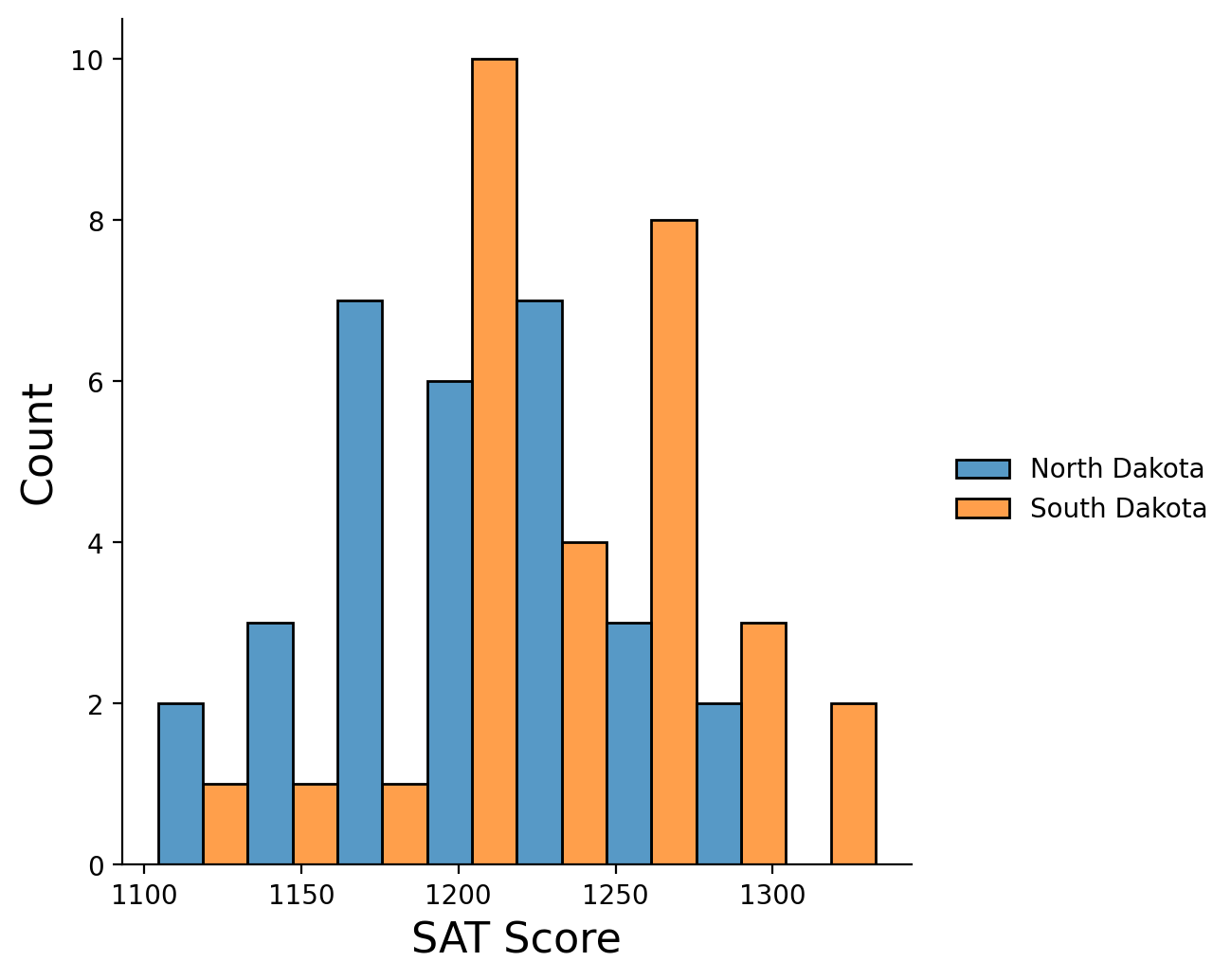
Under the Neyman-Pearson or NHST testing framework, our null hypothesis would be “students in North Dakota have the same average scores on the SAT as students in South Dakota.”
Now, almost certainly this is not true. That’s not the right question!
The important question is, in which state are scores higher, and how large is the difference – ie, what is the effect size?
Problem 2: Misunderstanding what a p-value is.
The p-value is the probability of getting our observed result, or a more extreme result, if the null hypothesis is true. So \(p\) is defined in relation to a stated null hypothesis, and requires as the basis for calculation that we assume the null is true.
It’s a common error to think \(p\) gives the probability that the null is true. Mistakenly thinking so is called the inverse probability fallacy. To do that, is to confuse \(p(\text{data}|H_0)\) with \(p(H_0|\text{data})\).
For example, if you are taking this course, there is a high probability you are a student a BU. But that does not mean that if you are a student at BU, there is a high probability you are taking this course.
Problem 3: Ignoring our Expertise or Prior Knowledge.
One of the ways in which standard NHST is flawed is in the standard use of 0.05 or 0.01 as a significance threshold. This fixed value of \(\alpha = 0.05\) or 0.01 in practice ignores what we know.
Consider a study in which researchers claim to detect 33 individuals out of 97 who show psychic ability, yielding a p-value of 0.047. By standard practice, this would be considered statistically significant since \(p < 0.05\). But given what we know about claims for psychic ability, are we really confident that the experiment shows that people have psychic abilities?
Another reason for avoiding a fixed significance threshold relates to our tolerance for false alarms. For example, particle physicists are particularly concerned with avoiding false alarms, which would trigger the development of new theories. So the standard for detection in particle physics is generally at least \(5\sigma\), corresponding to a p-value of about \(3 \times 10^{-7}\).
Problem 4: Downplaying False Negatives.
The standard NHST framework focuses on avoiding Type I errors (false positives). However if we fail to find statistical significance where there is a true effect, we are committing a Type II error (a false negative).
Unfortunately, often little attention is paid to Type II errors. A type II error can occur if an experiment does not collect enough data to establish small confidence intervals. This is called an underpowered experiment.
As a result, particularly when working with small datasets, we must be careful not to take statistical nonsignificance as evidence of a zero effect.
Have Confidence in Intervals#
In general, whenever possible, instead of using p-values to demonstrate statistical signficance, it is better to use confidence intervals.
For example, recall the example from the end of the last lecture:
height |
95% CI |
|
|---|---|---|
men, n = 25 |
69.0 in |
[68.1, 69.9] |
women, n = 23 |
61.1 in |
[60.3, 62.0] |
Notice that presenting confidence intervals avoids the problems associated with p-values and NHST.
We can easily see that the two groups have a statistically significant difference in means, because the confidence intervals do not overlap.
Furthermore, we can also easily see the effect size – the difference in average heights between men and women.