Joint Distributions

Today we’ll talk about joint distributions - distributions involving more than one random quantity.

Note

The majority of the examples come from Probabilistic Graphical Models,, Koller and Friedman, 2009, pages 20ff.

Let’s start with an example. Consider a distribution over a population of students in a course. Suppose we want to reason about how much students study, what grades they get, and other attributes of a student.

We’ll define categorical random variables StudyEffort and Grade, which are properties of students.

StudyEffort can take on the values low, and high. Grade can take on the values A, B, and C.

To fully characterize our student population, we need to specify the joint distribution of StudyEffort and Grade.

These are both categorical random variables, so the full distribution is a table.

For example, it could be:

\[ P(\text{Grade}, \text{StudyEffort}) = \]

	low	high
A	0.07	0.18
B	0.28	0.09
C	0.35	0.03

On the other hand, we could also be interested in each characteristic on its own. For example, we might be interested in the distribution of StudyEffort across our population.

This is called a marginal distribution.

It gets this name because it corresponds to the marginal sums of the probability distribution.

For example,

	low	high	marginal
A	0.07	0.18	0.25
B	0.28	0.09	0.37
C	0.35	0.03	0.38
marginal	0.70	0.30

The marginal for an attribute value is the sum of the probabilities over all possible values of all the other attributes.

So the marginal for Grade is the sum across the rows, and the marginal for StudyEffort is the sum across the columns.

Mathematically, we write:

\[ P(X) = \sum_y P(X, Y = y) \]

Or sometimes we would be even briefer:

\[ P(X) = \sum_Y P(X, Y) \]

(Be careful about this notation - make sure you understand when you read it that \(Y\) is taking on different values, but \(X\) is not.)

The same idea applies to numerical random variables. Let us first illustrate the concept on a simple example.

Assume that a fair coin is tossed three times. Let \(X\) denote the number of heads on the first toss and \(Y\) the total number of heads. The sample space is then equal to

\[\Omega = \{ HHH, HHT, HTH, HTT, THH, THT, TTH, TTT\}.\]

From the sample space we see that the joint probability mass (or frequency) function of \(X\) and \(Y\) is as given in the following table:

	\(y = 0\)	\(y = 1\)	\(y = 2\)	\(y = 3\)
\(x = 0\)	\(\frac{1}{8}\)	\(\frac{2}{8}\)	\(\frac{1}{8}\)	0
\(x = 1\)	0	\(\frac{1}{8}\)	\(\frac{2}{8}\)	\(\frac{1}{8}\)

Thus, \(p(0,2) = P(X=0, Y=2) = \frac{1}{8}.\)

Can you find the marginal frequency function of \(Y\)?

Let us look at another example. Here is a set of observations of two random variables, \(X_1\) and \(X_2\):

We can look at the joint distribution of the data and then calculate the marginals by summing over the joint probabilities.

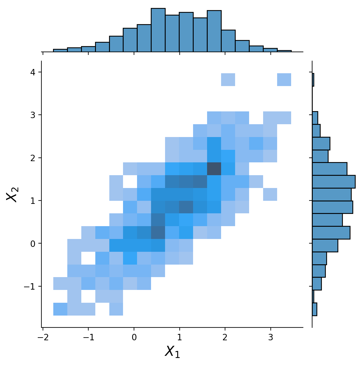
This plot summarizing the data shows:

• the two-dimensional distribution (i.e. joint probabilities) in the center (summarized in bins, darker is more dense)

• the two marginal distributions on the sides, as histograms (bar charts)

Let’s consider the the actual data again. If we were given the data points, rather than the joint probabilities, could we compute the marginals?

Yes! With observed data, the marginal distribution for an attribute can directly be found as the empirical distribution of that particular attribute while ignoring all others!

Independence

The Categorical Case

In a generic situation, if we want to specify a joint distribution, we need to specify the entire table of probabilities - one entry for each combination of possible values of the random variables.

To return to our previous example:

\[ P(\text{Grade}, \text{StudyEffort}) = \]

	low	high
A	0.07	0.18
B	0.28	0.09
C	0.35	0.03

Note as well that we found the following marginal distributions:

low	high
0.70	0.30

A	B	C
0.25	0.37	0.38

Let’s consider a new situation. Just for the purposes of discussion (and only for this purpose!) let’s imagine that the amount that a student studies has no effect on the grade that they get.

We would then say:

\[ P(\text{Grade}\,\mid\, \text{StudyEffort}) = P(\text{Grade}).\]

In other words, we would say that \(\text{StudyEffort}\) and \(\text{Grade}\) are independent.

In that case, we conclude that:

\[ P(\text{Grade}, \text{StudyEffort}) = P(\text{Grade})\cdot P(\text{Study Effort}).\]

Although looking at \(P(\text{Grade}, \text{StudyEffort})\) might be less intuitive than considering \(P(\text{Grade}\,\mid\, \text{StudyEffort})\), \(P(\text{Grade}, \text{StudyEffort})\) is the probability we need to work with to show that the variables are either dependent or independent.

Starting from the marginals

low	high
0.70	0.30

and

A	B	C
0.25	0.37	0.38

we can compute the new distribution (based on the independence assumption) as:

\[ P(\text{Grade}, \text{StudyEffort}) = \]

	low	high
A	0.175	0.075
B	0.259	0.111
C	0.266	0.114

The Numerical Case

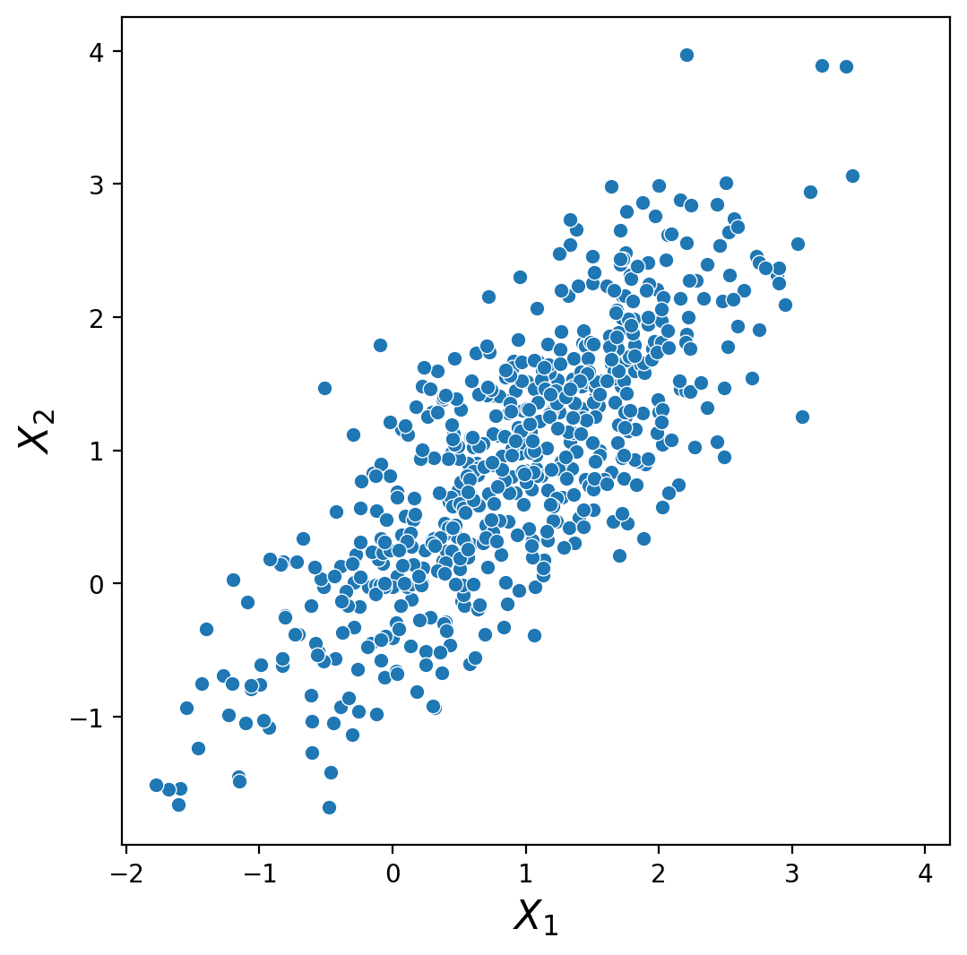
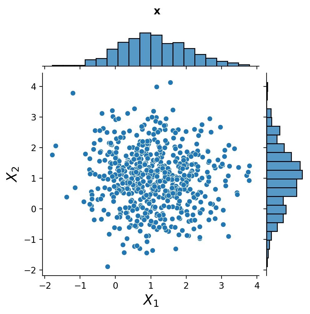
Now let’s look at one of our examples that involves numerical random variables.

Are \(X_1\) and \(X_2\) independent for this case?

No - it’s clear that if we know that \(X_2 > 1\) , then the probability that \(X_1 > 1\) increases.

That is,

\[ P(X_1 \text{ is large}\,\mid\,X_2 \text{ is large}) > P(X_1\text{ is large}) \]

so \(X_1\) and \(X_2\) are not independent.

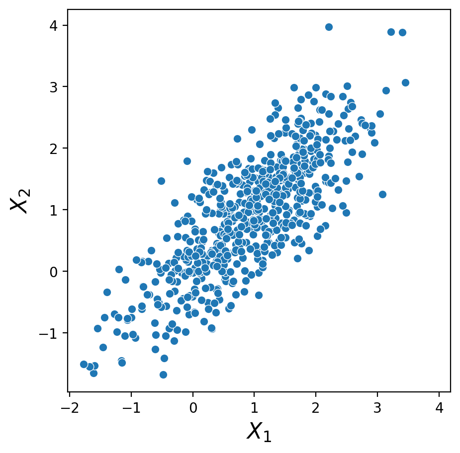
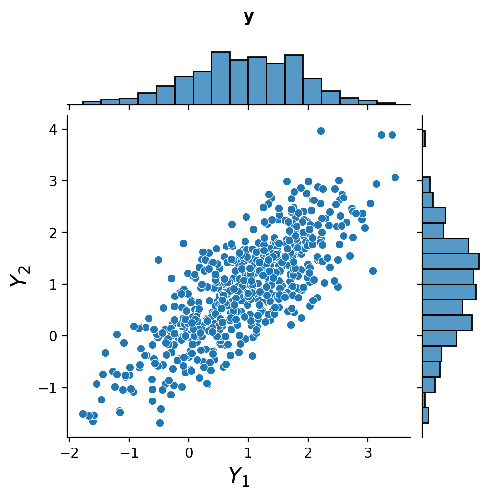
Now consider these two datasets:

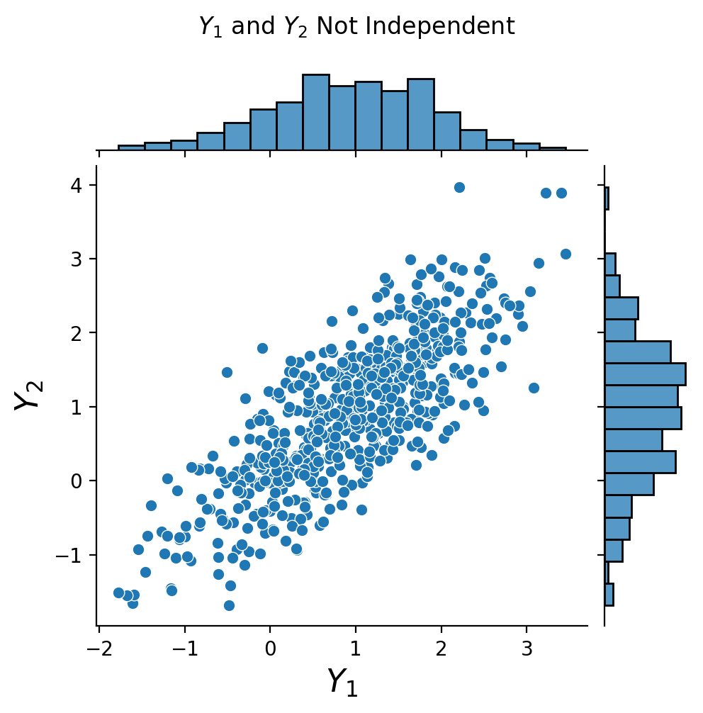
Notice that they have approximately the same marginals. However, for the first dataset, \(X_1\) and \(X_2\) are independent, but in the second case, \(Y_1\) and \(Y_2\) are not independent.

Correlation

To describe the lack of independence between \(X_1\) and \(X_2\) above, we’d need to show that

\[ p(x_1, x_2) = p_{X_1}(x_1)p_{X_2}(x_2).\]

for each value of \(x_1\) and \(x_2\).

However, in many cases this is a non-trivial task.

The most common way to describe a relationship between random variables with a single number is covariance.

Covariance extends the concept of variance to multiple random variables.

The covariance of \(X_1\) and \(X_2\), denoted \(\operatorname{Cov}(X_1, X_2)\) is defined as:

\[ \operatorname{Cov}(X_1, X_2) = E[(X_1 - \overline{X_1})(X_2 - \overline{X_2})] \]

where \(\overline{X_1}\) and \(\overline{X_2}\) are the means of \(X_1\) and \(X_2\).

We will often denote \(\operatorname{Cov}(X,Y)\) as \(\sigma_{XY}\).

Let’s look at a specific example. Here are the stock prices of two companies over a one-year period:

Clearly, these two stock prices are not independent.

This is in large part because both stocks respond to overall market conditions:

One way to describe these two stocks is that they are “likely to be above their respective means at the same time.”

That is, they “co-vary”.

This is what is captured by covariance.

We know how to find the expected value of a random variable. But how exactly do we compute

\[\operatorname{Cov}(X_1, X_2) = E[(X_1 - \overline{X_1})(X_2 - \overline{X_2})]?\]

For discrete \(X_1\) and \(X_2\) with joint probability \(P(X_1=x_1, X_2=x_2) = p(x_1,x_2)\) the covariance is computed as

\[ \operatorname{Cov}(X_1, X_2) = \sum_{(x_1,x_2)\in S} (x_1 - \overline{X_1})(x_2 - \overline{X_2}) p(x_1,x_2). \]

Here, \(S\) is the support of \(X_1\) and \(X_2\).

Note: The covariance of two continuous random variables is outside the scope of this course.

Let us look at a simple example.

Suppose that \(X\) and \(Y\) have the joint probability mass function given below.

	\(x = 5\)	\(x = 6\)	\(x = 7\)
\(y = 8\)	0	0.4	0.1
\(y = 9\)	0.3	0	0.2

In this case, the support \(S\) is equal to the set \(\{(5,8),(6,8),(7,8), (5,9),(6,9),(7,9)\}.\)

The marginal probabilities are given by

	\(x = 5\)	\(x = 6\)	\(x = 7\)
\(p_X(x)\)	0.3	0.4	0.3

	\(y = 8\)	\(y = 9\)
\(p_Y(y)\)	0.5	0.5

The mean of \(X\) can be computed using \(p_X(x)\) as follows

\[\overline{X} = 5 \cdot 0.3 + 6 \cdot 0.4 + 7 \cdot 0.3 = 6.\]

Similarly, we find that \(\overline{Y} = 8.5.\)

Now it remains to compute the covariance itself

\[\operatorname{Cov}(X,Y) = (5-6)(8-8.5)(0) + (6-6)(8-8.5)(0.4) + (7-6)(8-8.5)(0.1)\]

\[+ (5-6)(9-8.5)(0.3) + (6-6)(9-8.5)(0) + (7-6)(9-8.5)(0.2) = -0.1.\]

We typically “normalize” covariance by the standard deviations of the random variables.

This is called “correlation coefficient” or “Pearson’s correlation coefficient” or “Pearson’s \(\rho\)”:

\[\rho(X_1,X_2) = \frac{E\left[(X_1-\overline{X_1})(X_2-\overline{X_2})\right]}{\sigma_{X_1} \sigma_{X_2}}\]

As we will see later on, another way to think of correlation coefficient is:

“How well could a linear model predict one random variable, given the other?”

Because it is normalized, \(\rho(X_1, X_2)\) takes on values between -1 and 1.

If \(\rho(X_1, X_2) = 0\) then \(X_1\) and \(X_2\) are uncorrelated.

If \(\rho(X_1, X_2) > 0\) then \(X_1\) and \(X_2\) are positively correlated, and if \(\rho(X_1, X_2) < 0\) they are anticorrelated.

Now: (this is important!):

If \(X_1\) and \(X_2\) are uncorrelated, are they independent?

In general, NO.

If \(X_1\) and \(X_2\) are uncorrelated, that means the relationship between them can’t be predicted by a linear model.

However, this does not mean that they are necessarily independent!

Here is a rule of thumb when working with correlation:

• If \(X_1\), \(X_2\) are independent, then they have a zero correlation coefficient.

• If \(X_1\), \(X_2\) have a zero correlation coefficient, they are possibly, but not necessarily independent.

More generally, keep in mind that when you use Pearson’s \(\rho\), you are making a linear assumption about the data.

This can be highly misleading if you are not aware of the structure present in your data.

Note

This example is called Anscombe’s Quartet. Image source: https://en.wikipedia.org/wiki/Anscombe’s_quartet

Let’s look at a classic example of four datasets, each of which has the same correlation coefficient:

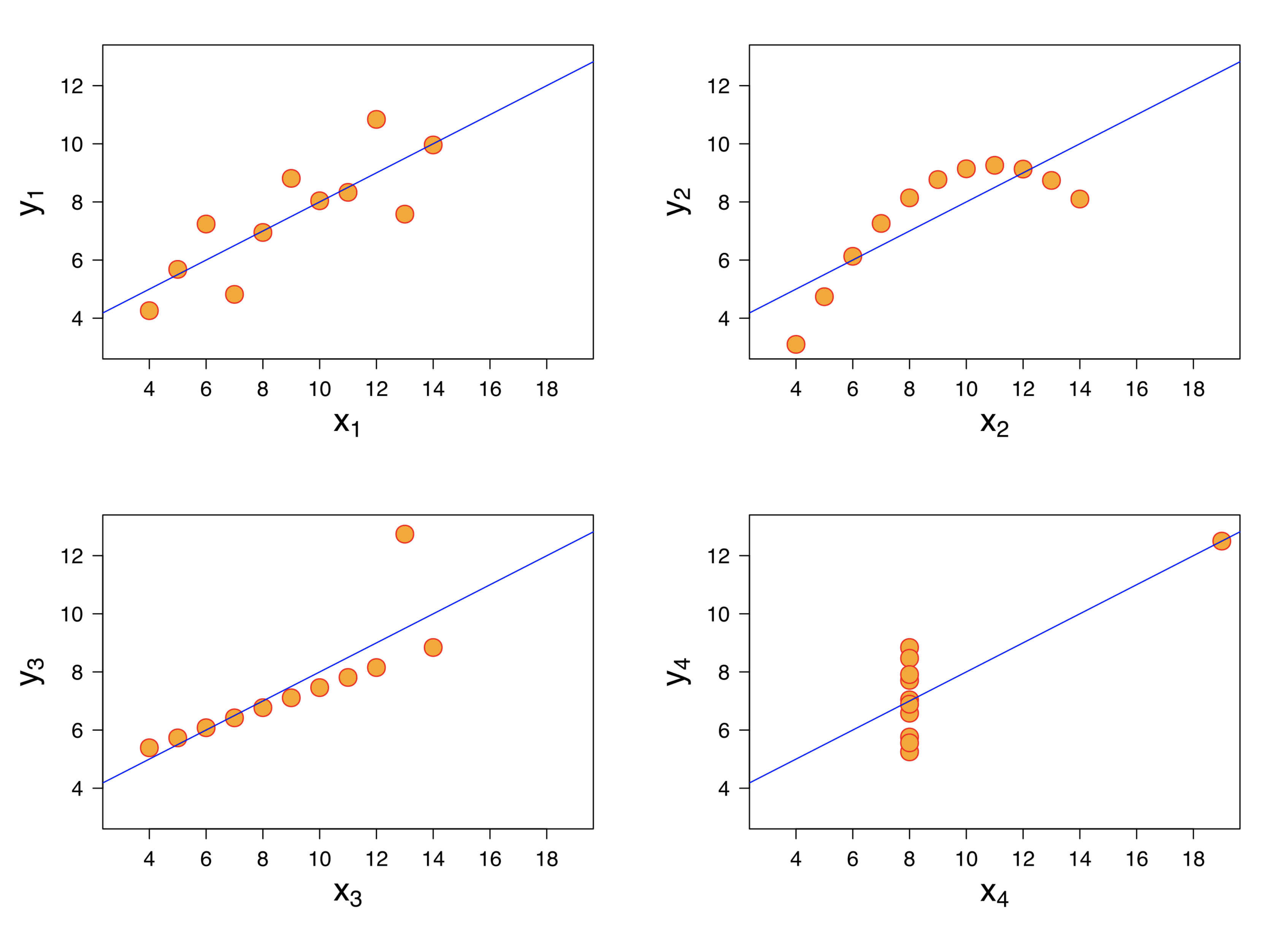
In this example, for the two datasets on the right, a linear model does not seem appropriate.

And for the dataset in the lower left, the linear model is misleading because of the outlier.

However all four datasets have the same correlation coefficient (0.816)!

This example shows the importance of looking at your data before beginning to analyze it.

Bonus material:

Random Vectors

We will often collect a set of random variables into a vector, naturally called a random vector.

To do this, we need to define the linear algebra of random vectors. This will be a straightforward extension of the usual notion of vectors.

Definitions

A random vector \(\mathbf{x}\) is a collection of random variables, denoted

\[\begin{split} \mathbf{x} = \left[\begin{array}{c}X_1\\X_2\\\vdots\\X_n\end{array}\right] \end{split}\]

In an experiment where we can measure random outcomes \(X_1\) and \(X_2\), we define the random variable \(X_1 + X_2\) to be the random outcome we get when we sum the measures \(X_1\) and \(X_2\).

In the frequentist interpretation of “independent trials under identical conditions”, each time we perform a trial we sum the values of \(X_1\) and \(X_2\) for that trial.

Likewise, we will define the product \(a X_1\), where \(a\) is a (non-random) scalar value, as the random variable corresponding to observing \(X_1\) and then multiplying that observation by \(a\).

With these definitions, we can construct a vector space as follows:

For

\[\begin{split}\mathbf{x} = \left[\begin{array}{c}X_1\\X_2\\\vdots\\X_n\end{array}\right] \text{ and } \mathbf{y} = \left[\begin{array}{c}Y_1\\Y_2\\\vdots\\Y_n\end{array}\right]\end{split}\]

We define:

\[\begin{split}\mathbf{x} + \mathbf{y} = \left[\begin{array}{c}X_1 + Y_1\\X_2 + Y_2\\\vdots\\X_n + Y_n\end{array}\right]\end{split}\]

\[\begin{split} a\mathbf{x} =\left[\begin{array}{c}aX_1\\aX_2\\\vdots\\aX_n\end{array}\right]\end{split}\]

Properties of Random Vectors

It is straightforward to define the expectation or mean of a random vector:

\[\begin{split} E[\mathbf{x}] = \left[\begin{array}{c}E[X_1]\\E[X_2]\\\vdots\\E[X_n]\end{array}\right] = \mathbf{\mu}. \end{split}\]

Note that \(\mathbf{\mu}\) is a vector, but it is not random (it is a “regular” vector).

What about variance?

It’s important to keep in mind that components of the random vector \(\mathbf{x}\) may be correlated.

So in general we want to know about all the possible correlations in \(\mathbf{x}\).

This leads us to define the covariance matrix:

\[\begin{split}\Sigma = \operatorname{Cov}(\mathbf{x}) = \left[\begin{array}{cccc} \sigma_{11}&\sigma_{12}&\dots&\sigma_{1n}\\ \sigma_{21}&\sigma_{22}&\dots&\sigma_{2n}\\ \vdots & \vdots & \ddots & \vdots\\ \sigma_{n1}&\sigma_{n2}&\dots&\sigma_{nn}\\ \end{array}\right]\end{split}\]

where \(\sigma_{ij} = \operatorname{Cov}(X_i, X_j)\).

Note that this definition implies that the variances of the components of \(\mathbf{x}\) lie on the diagonal of the covariance matrix \(\Sigma\).

That is, \(\sigma_{ii} = \operatorname{Var}(X_i).\)

A random vector is referred to as singular or nonsingular depending on whether its covariance matrix \(\Sigma\) is singular or nonsingular.

Let’s return to a previous example, and now interpret things in terms of random vectors.

We will say that \(\mathbf{x} = \left[\begin{array}{c}X_1\\X_2\end{array}\right]\)

Now, however, instead of thinking of these plots as scatterplots of \(X_1\) vs \(X_2\) observations, we think of each point as an observation of the random vector \(\mathbf{x}\) .

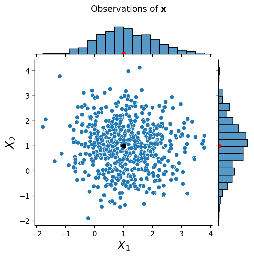
What is the mean of this random vector?

We’ve found the mean of each marginal (marked in red dots). Both marginals have mean 1.

So the mean of the random vector \(\mathbf{x}\) is

\[\begin{split}\mathbf{\mu_x} = \left[\begin{array}{c}E[X_1]\\E[X_2]\end{array}\right] = \left[\begin{array}{c}1\\1\end{array}\right].\end{split}\]

The mean \(\mathbf{\mu_x}\) is marked with a black dot.

What is the covariance matrix of this random vector?

When we compute the covariance matrix we get

\[\begin{split}\Sigma_\mathbf{x} = \left[\begin{array}{cc} \sigma_{11}&\sigma_{12}\\ \sigma_{21}&\sigma_{22}\\ \end{array}\right] = \left[\begin{array}{cc} 1&0\\ 0&1\\ \end{array}\right]\end{split}\]

The off-diagonal elements are zero, which is what we expect since we know that \(X_1\) and \(X_2\) are independent.

So when the components of a random vector are independent, its covariance matrix is a diagonal matrix.

Now, let’s also define \(\mathbf{y} = \left[\begin{array}{c}Y_1\\Y_2\end{array}\right]\).

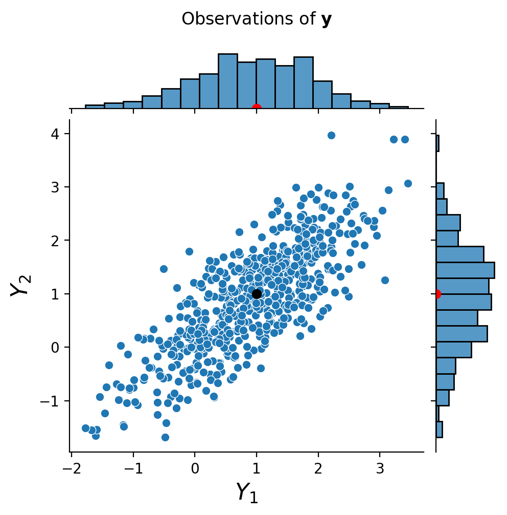
This random vector \(\mathbf{y}\) has that same mean as \(\mathbf{x}\):

\[\begin{split}\mathbf{\mu_y} = \left[\begin{array}{c}1\\1\end{array}\right].\end{split}\]

However the covariance matrix \(\Sigma_\mathbf{y}\) is quite different:

\[\begin{split}\Sigma_\mathbf{y} = \left[\begin{array}{cc} 1&0.8\\ 0.8&1\\ \end{array}\right]\end{split}\]

The off-diagonal elements of \(\Sigma_\mathbf{y}\) are nonzero, which is not surprising as we know that \(Y_1\) and \(Y_2\) are not independent.

Finally, we can ask whether \(\Sigma_\mathbf{y}\) is singular.

One way would be to compute its eigenvalues. (We could also check its determinant.)

We find that the eigenvalues of \(\Sigma_\mathbf{y}\) are 1.8 and 0.2. Since neither one is zero, we conclude that \(\Sigma_\mathbf{y}\) is nonsingular, and so \(\mathbf{y}\) is nonsingular.

So in general we conclude that:

• When the components of a random vector are independent, its covariance matrix is a diagonal matrix.

• When the components of a random vector are not independent, the covariance matrix will generally not be a diagonal matrix. (But remember, it is still possible – dependent random variables can have zero correlation!)

Multivariate Normal

A very commonly-encountered case will be a random vector that is multivariate normal or multivariate Gaussian.

Definition.

Let \(\mathbf{z} = \left[\begin{array}{c}Z_1\\\vdots\\Z_n\end{array}\right]\) where \(Z_1, \dots, Z_n\) are independent, identically-distributed (i.i.d.) normal (Gaussian) random variables having mean zero and unit variance.

Note that \(\mu_\mathbf{z} = \mathbf{0}\) and \(\Sigma_\mathbf{z} = I\).

Then we say that \(\mathbf{y}\) has an \(r\)-dimensional multivariate normal distribution if \(\mathbf{y}\) has the same distribution as \(A\mathbf{z} + \mathbf{b}\), for some \(r \times n\) matrix \(A\), and some vector \(b \in \mathbb{R}^r\).

In other words, each component of \(\mathbf{y}\) is a linear combination of standard normal random variables, plus a constant.

We indicate the multivariate normal distribution of \(\mathbf{y}\) by writing \(\mathbf{y} \sim N(\mathbf{b},AA^T)\).

As discussed previously, the central limit theorem tells us that the sum of normal random variables is also a normal random variable.

So, the components of \(\mathbf{y}\) are normal random variables.

Notice two key things here:

• the constant vector \(\mathbf{b}\) that we add becomes the mean vector of \(\mathbf{y}\).

• the covariance matrix \(\Sigma\) of \(\mathbf{y}\) is equal to \(AA^T\).

Example.

As it happens, the examples we have been using so far are actually examples of multivariate normal distributions.

We have

\[\mathbf{x} \sim N(\mathbf{\mu_x}, \Sigma_\mathbf{x})\]

where \(\mathbf{\mu_x} = \left[\begin{array}{c}1\\1\end{array}\right]\) and \(\Sigma_\mathbf{x} = \left[\begin{array}{cc} 1&0\\ 0&1\\ \end{array}\right]\),

and

\[\mathbf{y} \sim N(\mathbf{\mu_y}, \Sigma_\mathbf{y})\]

where \(\mathbf{\mu_y} = \left[\begin{array}{c}1\\1\end{array}\right]\) and \(\Sigma_\mathbf{y} = \left[\begin{array}{cc} 1&0.8\\ 0.8&1\\ \end{array}\right]\),

Notice that the marginal distributions are Gaussian.

An Important Property of the Multivariate Normal

One of the reasons that the multivariate normal is nice to work with is the following.

Theorem.

If \(\mathbf{y} \sim N(\mathbf{\mu}, \Sigma)\) and \(\mathbf{y} = \left[\begin{array}{c}Y_1\\Y_2\end{array}\right]\), then \(\operatorname{Cov}(Y_1, Y_2) = 0\) if and only if \(Y_1\) and \(Y_2\) are independent.

We will not prove this (though it’s not hard to prove.)

Note that what this theorem is saying is that multivariate normal is a special case.

Although \(\operatorname{Cov} = 0\) does not imply independence in general, for the multivariate normal, it does.

So we can conclude, whenever working with multivariate normals, that if a covariance term in \(\Sigma\) is zero, then the corresponding components are independent.