Gradients

A good reference for this section is Chapter 1 of Numerical Algorithms by Justin Solomon. A number of our examples are taken from there.

Over the next few lectures we will build from calculating gradients (which many of you have seen) to using gradient descent to find local maxima/minima, to exploring and implementing algorithms for gradient descent.

Review of Derivatives

The importance of the derivative is based on a simple but important observation.

While many functions are globally nonlinear, locally they exhibit linear behavior. This idea is one of the main motivators behind differential calculus.

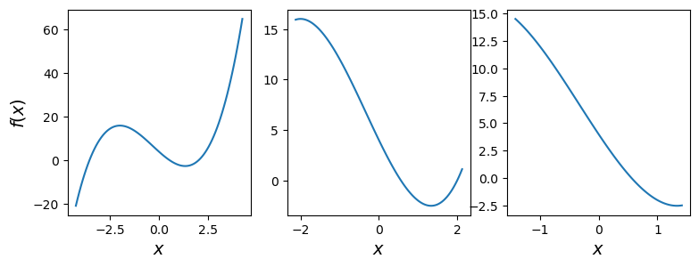
Consider this smooth function:

\[ f(x) = x^3 + x^2 - 8x + 4 \]

The closer we zoom in on it, the more it looks like a line.

The derivative \(f'(x)\) of a function \(f(x): \mathbb{R}\rightarrow\mathbb{R}\) is the slope of the approximating line, computed by finding the slope of lines through closer and closer points to \(x\):

\[ f'(x) = \lim_{y\rightarrow x}\frac{f(y)-f(x)}{y-x}. \]

In other words, the derivative of a function at a point is basically its slope at that point.

Partial Derviatives

Now, our goal is going to be to apply this notion of “slope” to functions of more than one variable – that is, functions of vectors.

If a function \(f\) takes multiple inputs, then it can be written

\[ f(\mathbf{x}): \mathbb{R}^n \rightarrow \mathbb{R} \text{ for }\mathbf{x} \in \mathbb{R}^n.\]

In other words, for each point \(\mathbf{x} = \begin{bmatrix}x_1\\\vdots\\x_n\end{bmatrix}\) in \(n\)-dimensional space, \(f\) assigns a single number \(f(x_1, \dots, x_n)\).

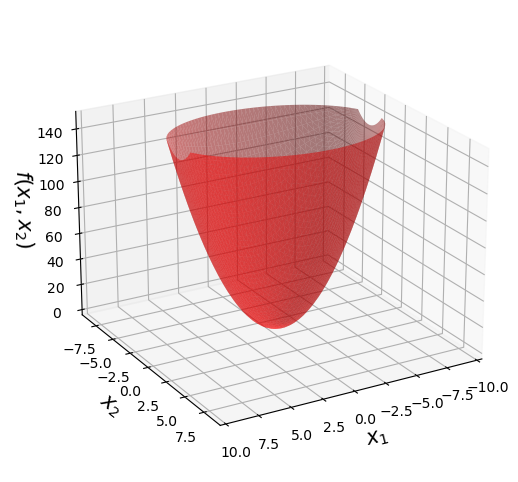
For example, for \(f(\mathbf{x}): \mathbb{R}^2 \rightarrow \mathbb{R}\), we can think of \(f\) as defining a surface in three dimensions.

Here is an example function:

\[ f(x_1, x_2) = 2 x_1^2 + 4 x_2^2 - 2 x_1x_2 + x_1 + x_2 + 3 \]

At first it may seem hard to apply the notion of linearity to a surface, since a line is a 1-D concept.

However, if we fix all but one variable, the function becomes a simple line again: \(\mathbb{R}\rightarrow\mathbb{R}\).

So we will isolate each variable and study it separately.

That means, we focus on one variable, and think of all other variables as constants.

This leads to a definition:

Partial Derivative. The partial derivative of \(f\) with respect to \(x\) is given by differentiating \(f\) with respect only to \(x\), holding the other inputs to \(f\) constant.

The partial derivative of \(f\) with respect to \(x\) is written

\[\frac{\partial f}{\partial x}\]

For example, consider the \(f\) above:

\[ f(x_1, x_2) = 2 x_1^2 + 4 x_2^2 - 2 x_1x_2 + x_1 + x_2 + 3 \]

To take the partial derivative of \(f\) with respect to \(x_1\), treat the occurrences of \(x_2\) as if they were “just numbers”.

So

\[ \frac{\partial f}{\partial x_1} = 4x_1 -2x_2 + 1 \]

And

\[ \frac{\partial f}{\partial x_2} = 8x_2 -2x_1 + 1 \]

Here is a visualization of the partial derivative with respect to \(x_1\).

Consider the case where \(x_2 = 3.\) Then we are looking at the 1D curve defined by the intersection of the plane \(x_2 = 3\) and the function \(f\).

Once Loop Reflect

Now, for this 1D curve lying in the plane, we can take its slope at any point. That is the meaning of the partial derivative

\[ \frac{\partial f}{\partial x_1} = 4x_1 -2x_2 + 1 \]

evaluated at \(x_2 = 3\).

The slope of the straight line in this figure is \(\frac{\partial f}{\partial x_1}\) at \(x_1 = 5, x_2 = 3.\)

Once Loop Reflect

Gradients

A single partial derivative tells you how the function is varying along a single dimension.

However, we often would like to get a sense of how the function is varying across all dimensions simultaneously.

We do this by collecting all the partial derivatives of the function into a vector called the gradient.

Definition.

Given a function \(f(\mathbf{x}): \mathbb{R}^n \rightarrow \mathbb{R} \text{ for }\mathbf{x} \in \mathbb{R}^n\) the gradient of \(f\) is defined as the vector of its partial derivatives:

\[\begin{split} \nabla_\mathbf{x}f = \begin{bmatrix} \frac{\partial f}{\partial x_1}\\ \vdots \\ \frac{\partial f}{\partial x_n} \end{bmatrix} \end{split}\]

Continuing our example, for \(\mathbf{x} \in \mathbb{R}^2\):

\[ f(\mathbf{x}) = 2 x_1^2 + 4 x_2^2 - 2 x_1x_2 + x_1 + x_2 + 3 \]

We have

\[\begin{split} \nabla_\mathbf{x}f = \begin{bmatrix} 4x_1 -2x_2 + 1 \\ 8x_2 -2x_1 + 1 \end{bmatrix} \end{split}\]

Note that the gradient of a function has the same shape as the function’s input. In other words, if \(\mathbf{x} \in \mathbb{R}^n\), then \(\nabla_\mathbf{x}f \in \mathbb{R}^n.\)

Examples.

Consider

\[f(x,y) = \sin(xy).\]

What is the gradient of \(f\)?

Answer: We need to find \(\partial f/\partial x\) and \(\partial f/\partial y\).

To find \(\partial f/\partial x\), treat y as a constant. So you can see that

\[\frac{\partial f}{\partial x} = y \cos(xy).\]

Likewise

\[\frac{\partial f}{\partial y} = x \cos(xy).\]

So

\[\begin{split} \nabla f = \begin{bmatrix} y \cos(xy) \\ x \cos(xy)\end{bmatrix}.\end{split}\]

Consider

\[f(x, y) = x^y.\]

What is the gradient of \(f\)?

Answer:

Treating \(y\) as a constant, we have

\[\frac{\partial f}{\partial x} = y x^{y-1}.\]

and treating \(x\) as a constant, we have

\[\frac{\partial f}{\partial y} = \ln x \cdot x^y.\]

So

\[\begin{split} \nabla f = \begin{bmatrix} y x^{y-1} \\ \ln x \cdot x^y\end{bmatrix}.\end{split}\]

Example: linear function of \(\mathbf{x}\)

A common case is when we have a linear function of a vector \(\mathbf{x}\).

That is, consider

\[ f(\mathbf{x}) = a_1 x_1 + a_2 x_2 + \dots + a_n x_n + b \]

A more concise way to write this is:

\[ f(\mathbf{x}) = \mathbf{a}^T\mathbf{x} + b \]

Where the coefficients \(a_1, \dots, a_n\) are collected into the vector \(\mathbf{a}\).

What is \(\nabla_\mathbf{x} f\)?

For a given term \(x_i\) in \(a_1 x_1 + a_2 x_2 + \dots + a_n x_n\), the corresponding partial derivative is just \(a_i\).

So \(\nabla_\mathbf{x} f = \mathbf{a}.\)

In other words, the gradient

\[ \nabla_\mathbf{x} (\mathbf{a}^T\mathbf{x} + b) = \mathbf{a} \]

Follows the same pattern as the familiar single variable case:

\[ \frac{d}{dx} ax+b = a.\]

(The only fine point to notice is that the gradient \(\mathbf{a}\) is the transpose of \(\mathbf{a}^T\).)

Steepest Ascent

One important question that gradients solve is the following:

Imagine we have some point, for example (5, 3), in the \((x_1, x_2)\) plane, and we have the same function from before

\[ f(x_1, x_2) = 2 x_1^2 + 4 x_2^2 - 2 x_1x_2 + x_1 + x_2 + 3 \]

Now assume we can move a unit distance (a distance of 1) in any direction in the \((x_1, x_2)\) plane.

What direction would we move in to cause the greatest increase in \(f\)?

In other words, we are asking, for a given point, what is the direction of steepest ascent?

To answer this question, let’s imagine we take a tiny step in the direction given by the vector \(d\mathbf{v} = (dv_1, dv_2).\)

This can be thought of as a step of length \(dv_1\) in the \(x_1\) direction, combined with a step of length \(dv_2\) in the \(x_2\) direction.

So the amount of change in \(f\) due to this tiny step is

\[dv_1 \cdot \frac{\partial f}{\partial x_1} + dv_2 \cdot \frac{\partial f}{\partial x_2}.\]

Note that this expression is actually the inner product of \(d\mathbf{v}\) with the gradient.

Expressed in vector terms, the amount of change is

\[d\mathbf{v}^T \nabla_\mathbf{x}.\]

Now, in what direction is \(d\mathbf{v}^T \nabla_\mathbf{x}\) maximized?

From linear algebra, we know that the inner product is proportional to the cosine of the angle between the vectors (i.e. that \(\mathbf{v} \cdot \mathbf{u}=||\mathbf{v}|| ||\mathbf{u}|| \cos(\theta)\)).

So the inner product is maximized when the angle is zero, that is, when \(d\mathbf{v}\) points in the same direction as the gradient.

So the answer is, the direction of steepest ascent is given by the gradient.

The gradient at (5,3) is plotted below, and the line points in the direction of steepest ascent on the surface above it.

Once Loop Reflect

When the Gradient is Zero

Consider a function \(f(\mathbf{x}): \mathbb{R}^n \rightarrow \mathbb{R}.\) Consider some “region” (some open set of \(\mathbb{R}^n\)). If \(f\) has a minimum or a maximum in the interior of that region, then all partial derivatives of \(f\) are zero.

You can see that this must be true, because if the gradient is nonzero, then a small step in some direction will increase \(f\), and a step in the opposite direction will decrease \(f\).

So at a local minimum or maximum, the gradient is zero.

Note that a local minimum could be a global minimum if there is no other point where \(f\) has a smaller value.

Unfortunately, the converse is definitely not true.

The fact that the gradient is zero at a point \(\mathbf{x}\) does not mean that \(f\) has a minimum or maximum at that point.

Any point where the gradient is zero, but the function does not have a local maximum or minimum, is called a saddle point.

The reason for this term comes from this example. Here is a point where the gradient is zero:

Quadratic Forms

Now we want to introduce a commonly encountered function, called a quadratic form.

A simple description of a quadratic form is that is a generalization of a quadratic function to vectors.

Definition. A quadratic form is a function of variables, eg, \(x_1, x_2, \dots, x_n,\) in which every term has degree two.

Examples:

\(4x_1^2 + 2x_1x_2 + 3x_2^2\) is a quadratic form.

\(4x_1^2 + 2x_1\) is not a quadratic form.

Quadratic forms arise in many settings, including signal processing, physics, economics, and statistics.

In computer science, quadratic forms arise in optimization and graph theory, among other areas.

Essentially, what an expression like \(x^2\) is to a scalar, a quadratic form is to a vector.

Every quadratic form can be expressed as \(\mathbf{x}^TA\mathbf{x}\), where \(A\) is a symmetric matrix.

There is a simple way to go from a quadratic form to a symmetric matrix, and vice versa.

To see this, let’s look at some examples.

Example. Let \(\mathbf{x} = \begin{bmatrix}x_1\\x_2\end{bmatrix}.\) Compute \(\mathbf{x}^TA\mathbf{x}\) for the matrix \(A = \begin{bmatrix}4&0\\0&3\end{bmatrix}.\)

Solution.

\[\begin{split}\mathbf{x}^TA\mathbf{x} = \begin{bmatrix}x_1&x_2\end{bmatrix}\begin{bmatrix}4&0\\0&3\end{bmatrix}\begin{bmatrix}x_1\\x_2\end{bmatrix}\end{split}\]

\[\begin{split}= \begin{bmatrix}x_1&x_2\end{bmatrix}\begin{bmatrix}4x_1\\3x_2\end{bmatrix}\end{split}\]

\[= 4x_1^2 + 3x_2^2.\]

Example. Compute \(\mathbf{x}^TA\mathbf{x}\) for the matrix \(A = \begin{bmatrix}3&-2\\-2&7\end{bmatrix}.\)

Solution.

\[\begin{split}\mathbf{x}^TA\mathbf{x} = \begin{bmatrix}x_1&x_2\end{bmatrix}\begin{bmatrix}3&-2\\-2&7\end{bmatrix}\begin{bmatrix}x_1\\x_2\end{bmatrix}\end{split}\]

\[=x_1(3x_1 - 2x_2) + x_2(-2x_1 + 7x_2)\]

\[=3x_1^2-2x_1x_2-2x_2x_1+7x_2^2\]

\[=3x_1^2-4x_1x_2+7x_2^2\]

Notice the simple structure:

\[a_{11} \mbox{ is multiplied by } x_1 x_1\]

\[a_{12} \mbox{ is multiplied by } x_1 x_2\]

\[a_{21} \mbox{ is multiplied by } x_2 x_1\]

\[a_{22} \mbox{ is multiplied by } x_2 x_2\]

We can write this concisely:

\[ \mathbf{x}^TA\mathbf{x} = \sum_{ij} a_{ij}x_i x_j \]

Quadratic Forms, Visually

Let’s look at some example quadratic forms:

Here is \(2x_1^2 + 3 x_2^2\).

Its matrix form is \(\mathbf{x}^TA\mathbf{x}\) with \(A = \begin{bmatrix}2&0\\0&3\end{bmatrix}.\)

You can see the parabolic shape which we expect since this is a generalization of the parabola.

Another kind of quadratic form is \(-3x_1^2 - 2 x_2^2\).

Its matrix form is \(\mathbf{x}^TA\mathbf{x}\) with \(A = \begin{bmatrix}-3&0\\0&-2\end{bmatrix}.\)

Another kind of quadratic form is shown below.

Quadratic Forms are Common

Quadratic forms show up often in machine learning and statistics.

For example, consider a linear regression, in which we are trying to predict observations \(\mathbf{y}\) using coefficient matrix \(\beta\) applied to unknowns \(\mathbf{x}\).

We seek to minimize

\[\Vert \beta\mathbf{x} - \mathbf{y}\Vert^2.\]

Since we know that the definition of \(\Vert \mathbf{w}\Vert^2 = \mathbf{w}^T\mathbf{w}\), we see that the expression we want to minimize is

\[ \mathbf{x}^T\beta^T\beta\mathbf{x} - 2\mathbf{y}^T\beta\mathbf{x} + \mathbf{y}^T\mathbf{y}.\]

Notice that \(\mathbf{x}^T\beta^T\beta\mathbf{x}\) is a quadratic form.

Gradient of Quadratic Form

Since they are so important, it can be useful to be able to compute the gradient of a quadratic form.

It’s actually not hard to do.

Recall that another way to write \(\mathbf{x}^TA\mathbf{x}\) is \(\sum_{ij} a_{ij}x_i x_j \)

Let’s consider just the partial derivative with respect to \(x_1\):

\[ \frac{\partial}{\partial x_1} \sum_{ij} a_{ij}x_i x_j .\]

We can throw out all the terms in which \(x_1\) does not appear because they are constants that disappear in the derivative. We are left with:

\[ \sum_k a_{1k} x_k + \sum_k a_{k1} x_k \]

Note that because \(A\) is symmetric, \(a_{1k} = a_{k1}\), so the two terms are equal:

\[ \frac{\partial}{\partial x_1} = 2\sum_k a_{1k} x_k \]

So the \(i\)th component of the gradient is twice the inner product of row \(i\) of \(A\) with \(\mathbf{x}\).

In other words, the gradient is just \(2A\) times \(\mathbf{x}\).

So:

\[ \nabla_\mathbf{x} (\mathbf{x}^TA\mathbf{x}) = 2A\mathbf{x}. \]

This is nice and simple. Notice how it parallels the case for single variables, ie, \(\frac{d}{dx} ax^2 = 2ax.\)

Example: Solving a Least-Squares Problem

As an example of putting all this together, let’s return to our example of solving a linear system by least squares. As mentioned earlier, we want to minimize

\[f(\mathbf{x}) = \Vert \beta\mathbf{x} - \mathbf{y}\Vert^2.\]

And this is the same as

\[f(\mathbf{x}) = \mathbf{x}^T\beta^T\beta\mathbf{x} - 2\mathbf{y}^T\mathbf{\beta}\mathbf{x} + \mathbf{y}^T\mathbf{y}.\]

Now, let’s find the gradient of this expression.

The gradient of the quadratic form term is

\[ \nabla_\mathbf{x} (\mathbf{x}^T\beta^T\beta\mathbf{x}) = 2\beta^T\beta\mathbf{x}.\]

And the gradient of the linear function terms is

\[ \nabla_\mathbf{x} (2\mathbf{y}^T\mathbf{\beta}\mathbf{x} + \mathbf{y}^T\mathbf{y}) = 2\beta^T\mathbf{y}.\]

So the complete gradient is:

\[ \nabla_\mathbf{x} f(\mathbf{x}) = 2\beta^T\beta\mathbf{x} - 2\beta^T\mathbf{y}\]

To solve the problem (ie find the minimum), let’s assume that there is a single global minimum.

Then we can find that minimum by setting the gradient to zero.

\[ \nabla_\mathbf{x} f(\mathbf{x}) = 2\beta^T\beta\mathbf{x} - 2\beta^T\mathbf{y}= 0 \]

So

\[ \beta^T\beta\mathbf{x} = \beta^T\mathbf{y}\]

Which we recogize as the normal equations for solving a least squares problem.

So (assuming \(\beta^T\beta\) is invertible):

\[ \mathbf{x} = (\beta^T\beta)^{-1}\beta^T\mathbf{y}\]

Which is the standard solution of a least squares problem.