Hypothesis Testing in Practice
Contents
Bonus material:
Hypothesis Testing in Practice#
Recall that the \(p\)-value is the probability of obtaining test results at least as extreme as the result actually observed, under the assumption that the null hypothesis is correct.
“Null Hypothesis Significance Testing” or NHST is the process of setting a \(p\)-value threshold and running a statistical test to see if you can reject the null hypthesis at that threshold. We suggested avoiding it because it is widely missused.
Overview of Statistical Tests#
However, in practice, you will sometimes perform standard hypothesis tests, so today we’ll run through some examples so that at the very least the tests are being used correctly. But think of this lecture more as a warning than as advice for how to navigate the world of data.
A huge variety of statistical tests has been developed to test various null hypotheses, each with specific assumptions about the data.
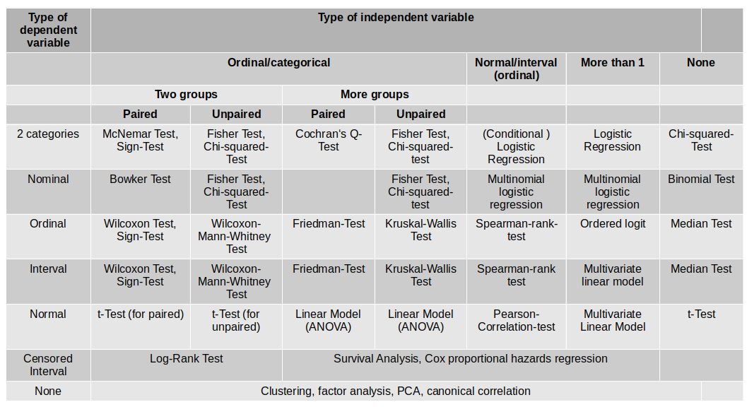
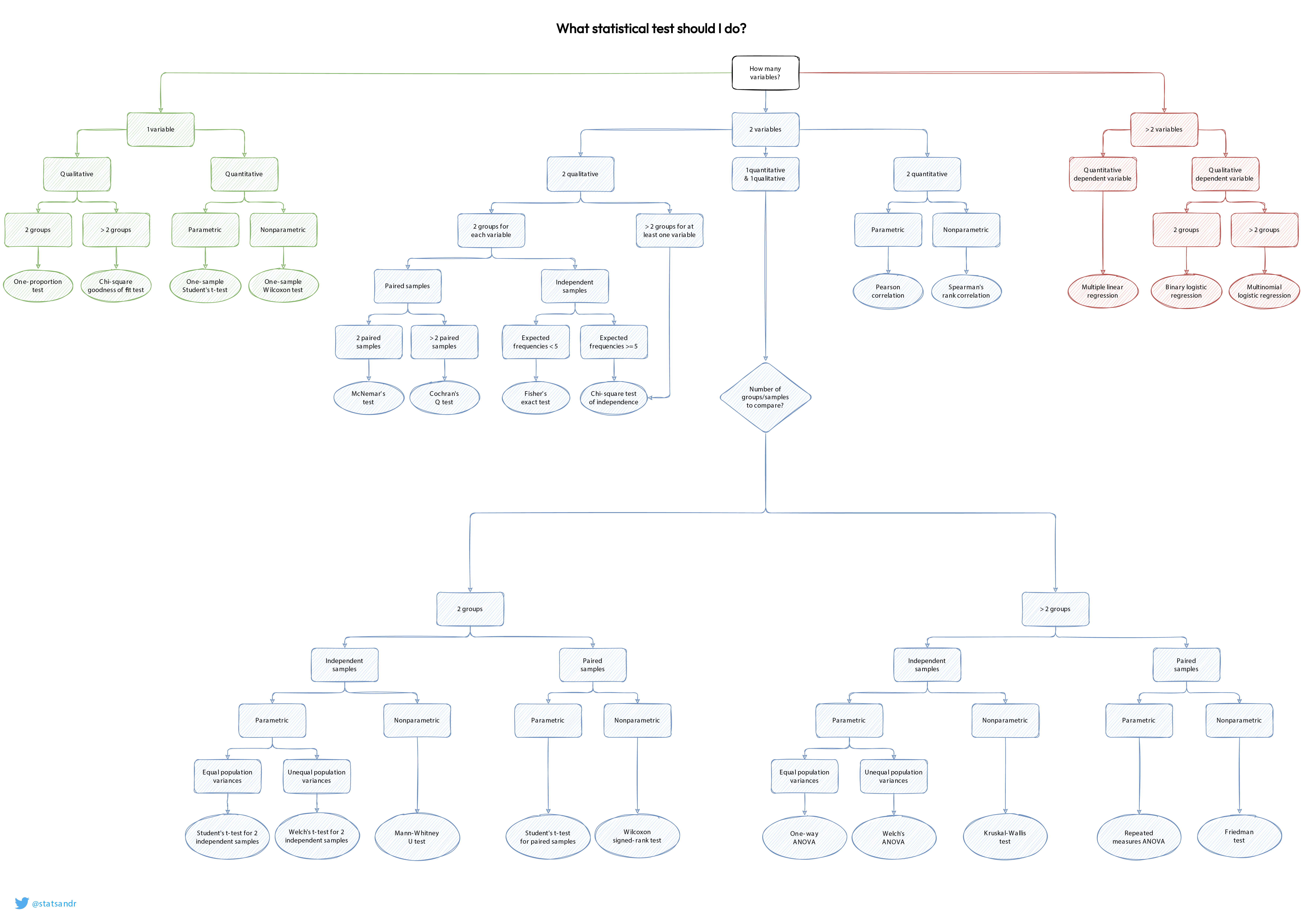
Picking the right test#
In fact, picking the right test is often so complicated, people make charts to help you choose:
Testing if there is a difference between two populations#
What if we wanted to test if there is a difference between two populations? For example, are men a different height than women on average? Well we actually already have all the tools necessary from the standard error calculations.
Fundementally, the question we can ask is “do the means of our samples of our populations lie within certain distances from each other?” and express those distances using standard errors.
To get at this we calculate the difference between the means and the standard error of the difference. The difference in means is straighforward:
but what about the standard error?
We know that for (independent random variables):
So then:
And we can use that to test our hypothesis.
One way we can do this is to check if the 95% confidence interval (or whatever level of confidence we would like to establish) includes 0. As we saw before, that means using a z-statistic. (We use 1.96 for a 95% CI.)
Another way is to directly calculate a p-value.
We can test the null hypothesis “How likely are we to see a difference in means as large as the one as we saw if we assume the true difference is 0.”
The distribution of differences in means is normal so this is a “z-test.”
A z-score (sometimes called a standard score) is calculated as:
The z-score can then be looked up in a table to find the corresponding p-value.
In our case, we would be calculating a z-score for \( x = 0, \mu = E[A] - E[B], \sigma = \text{SE}_{\text{A-B}}\), but z-scores can be used for testing the signficances of arbitrary values of x for some mean \(\mu\) and standard deviation \(\sigma\) of a normal distribution.
A note on being careful with z-scores:
There is a difference between simply asking if a particular value is far from the mean of a normal distribution with some known standard deviation, or if the question is about a sample mean from a population (i.e. is x a single value or a mean). In the first case we use the known standard deviation in the denominator, and in the latter we use the standard error because we are asking about the distribution of sample means.
Example#
Equipped with those equations, lets try to test if there is a difference based on a sample of heights of men and women. Both samples have more than 30 data points, so we can make use of the z-score. First, let’s compute the 95% confidence interval of the difference:
male_heights = np.array([216, 210, 213, 222, 152, 176, 220, 207, 209, 203, 193, 142, 135, 134, 205, 199, 149, 192, 172, 145, 167, 211, 179, 174, 133, 162, 135, 211, 142, 210, 168, 206, 190, 211, 179, 179, 178, 167, 148, 211])
female_heights = np.array([150, 132, 151, 121, 176, 142, 174, 166, 174, 125, 128, 150, 121, 189, 189, 149, 139, 177, 120, 157, 156, 169, 166, 160, 152, 142, 179, 180, 158, 151, 193, 173, 191, 223, 131, 178, 216, 105, 126, 165, 164, 180, 184, 152, 136, 170, 164, 194, 124, 127])

#Calculate the differene in means and the standard error of the difference
diff_in_means = np.mean(male_heights)-np.mean(female_heights)
se_of_diff = np.sqrt(np.std(male_heights)**2/len(male_heights)+np.std(female_heights)**2/len(female_heights)) #note: for simplicity this uses biased estimate of sd

# Calculate the 95% confidence interval
print(diff_in_means-1.96*se_of_diff,diff_in_means+1.96*se_of_diff)
11.350783659756452 33.839216340243546
So we see that 0 isn’t inside the 95% confidence interval.
Now let’s run a “z-test”, which means calculate the z-score and look up its corresponding p-value.
# Calculate and look up the z-score
from scipy.stats import norm
z_score = (0-diff_in_means)/se_of_diff #can be thought of as converting to a standard normal
norm.cdf(z_score)
4.098332516956473e-05
Looking up our z-score tells us there was a 0.004% chance of seeing a difference in means as extreme as the one we saw, if we assume the true difference is 0. This is far below typical NHST thresholds, so we would reject the null hypothesis.
What if we are working with smaller sample sizes?
Before we also touched on calculating the standard error for smaller populations using t-distribution that was introduced by William Gosset.
The history of the “t-distrubution” and the associated “t-test” often called the “Student’s t-test” is quite interesting. A man named William Gosset worked at the Guinness Brewery in Ireland and he needed a way determine if changes in the brewing processes made a difference. But unfortunately they generally only had small samples sizes (i.e. fewer than 30 beers per test).

He realized that he couldn’t use the standard procedure we described before because for small samples the uncertainty in estimating the standard error needs to be accouted for. We therefore need a distrubtion with “fatter” tails depending on the size of the sample, the result is the t-distrubution:
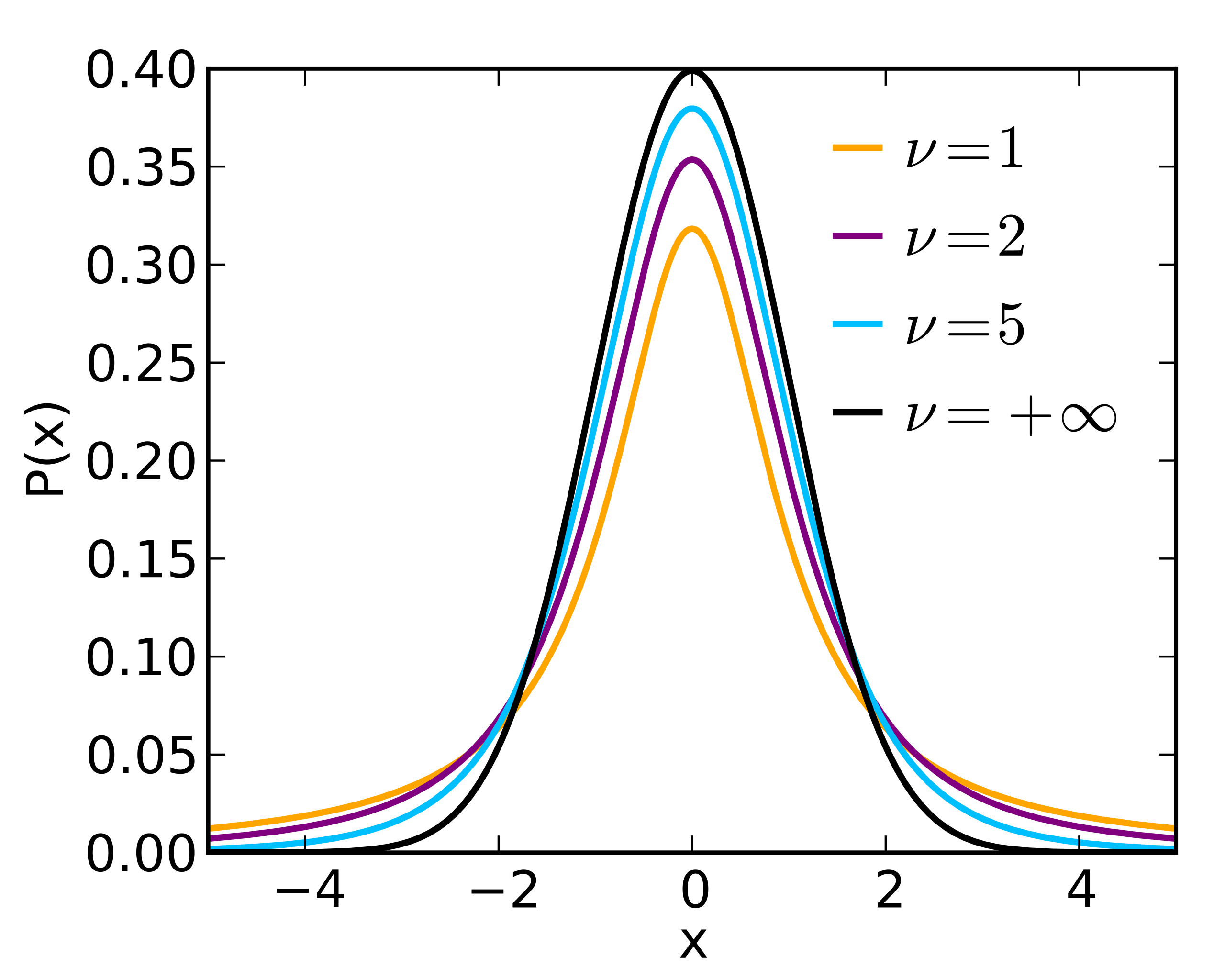
You can even see that as v (the degres of freedom, v=n-1) goes to infinity, we get the normal distribution.
Why is it called the Student’s t-test? The (probably false) story goes that Guinness did not want their competitors to know that they were using the t-test, so they forced Gosset to publish his work under the pseudonym.
Example#
Let’s follow Gosset’s ideas and see if adding barley changes the aciditiy of beer. We only have the measurements of acidities for 3 beers with barley and 4 without, so a t-test is appropriate.
barley_acidity = np.array([5,6,4])
no_barley_acidity = np.array([7,8,7,7])

#Calculate and look up the t-statistic
from scipy.stats import ttest_ind
ttest_ind(barley_acidity,no_barley_acidity)
Ttest_indResult(statistic=-3.9723067327713735, pvalue=0.010611745107949374)
This one line of code calculates the t-statistic for the difference between these two lists of numbers and the calculates the corresponding p-value.
That leads to the second note on being careful:
Remember that z-scores apply for normal distributions. We often say the sample means for a sample of size \(n \geq 30\) are normally distributed. However, if the sample size is smaller or we don’t know anything about the original distribution of the population, what we actually compute using the z-score formula is called a t-statistic, and needs to be looked up in a t-table for n-1 degrees of freedom (this is due to using the estimate s in place of the true \(\sigma\) of the population).
The Warning:#
In practice, much NHST is done with simple one-liners such as this, and the p-values are taken at face value. While it’s a usefull skill to have, we strongly recommend the confidence interval approach introduced in previous lectures. In fact, using one-liners like this can be dangerous since we often don’t fully understand the statistical test that is being conducted and what the underlying assumptions are.
You will see a lot of p-values and hypothesis testing in MA213/214, so that’s all NHST we are going to cover in DS122. Instead we will dive into the issues and potential abuse that naturally arises with the ease with which hypothesis testing can be applied.