Multiple Hypothesis Testing
Contents
Bonus material:
Multiple Hypothesis Testing#
Review of Hypthesis Testing#
Recall that we originally discussed two main framewoarks for hypthesis testing:
Fisher’s p-value: The p-value is the probability of obtaining test results at least as extreme as the result actually observed, under the assumption that the null hypothesis is correct.
The Neyman-Pearson Approach: We want to control the false positive rate \(\alpha\) to avoid making incorrect “discoveries.” The key concepts in this approach are:
False Positives (Type I Error) which are a mistaken rejection of the null hypothesis.
False Negatives (Type II Error) where we err by concluding that there is no difference when in fact there is a difference.
In this lecture we’ll look at how these approaches can be missued and used in the real world.
p-hacking#
One fundemental way p-values can be misued is that we interpret them as evaluations of independent hypotheses. However, what if we started violating that assumption.
Imagine you were flipping a coin to determine if it’s fair and you couldn’t reject the null hypotehsis given your series of coin flips. But what if you were determined to show the coin is not fair? You might decide to look for other ways to show the coin isn’t fair.
Consider the folowing series of coin flips: T T H T T H T T H H H T T H H H H
It came up close 50/50 heads and tails, so it looks lke a pretty fair coin.
Idea one
Maybe early in your flipping there had been an imbalance in the number of heads, and you chose where in the flips to stop counting to get a significant p-value. Looking at our coin flips above, maybe we decide we really only got the hang of flipping a coin after 8 warm-up flips.
Now our data looks like: H H H T T H H H H
That looks like an unfair coin!
Idea two
Maybe you change the criteria for what a fair coin looks like. Instead of having an equal number of heads or tails, it’s now determined by how many consecutive streaks of heads or tails there were. After all, a fair coin shouldn’t be streaky should it? Let’s say streaks of length 3 or longer are unusual.
Now our data looks like: Heads 2, Tails 0.
Pretty small sample size, but looks like it might not be a fair coin!
Idea three
Do coin flips really follow a Binomial distribution? What if you ran a statistical test and couldn’t reject the null hypthesis. So instead you chose something with a very narrow variance such that one more head than tails in a series of coin flips did turn out significant? This can be done for example by using a z-test instead of a t-test on a distribution with few samples.
There are many ways to p-hack. The main similarity is that we are no longer considering independent hypotheses! You might eventually slice and dice the data in a way that gives you a “significant” p-value, but that doesn’t actually mean you can reject the null hypothesis anymore.
Similarly, you might decide now to switch to a different hypothesis. Maybe it’s not that the coin isn’t fair, but that it isn’t fair when flipped on Tuesdays (assuming you had been flipping the coin for many days). Or Maybe it’s only on Tuesdays when you wear red? These just aren’t independent hypotheses anymore. They violate the fundemental principle of choosing the hypothesis and the test, and then collecting the data.
Multiple Hypothesis Testing#
You may encounter a slightly different scenario as well. It is very common in the real world to test many hypothesis at once. This leads to a second fundemtal problem:
So what went wrong there? What we are seeing is most likely a false positive. As we have discussed, the p-value tells you for a single experiment, what is the probability of seeing a value as extreme as the one you saw, given your assummptions. But that means (almost by definition) that if you do the same experiment enough times, one of those times you will have a signficant p-value.
A way to think about this is in terms of the number of hyptheses we have tested:
Test vs reality |
Null hypothesis is true |
…is false |
Total |
|---|---|---|---|
Rejected |
V |
S |
R |
Not rejected |
U |
T |
m−R |
Total |
m0 |
m−m0 |
m |
m - total number of hypotheses
m0 - number of true null hypotheses
V - number of false positives (a measure of type I error)
T - number of false negatives (a measure of type II error)
S, U - number of true positives and true negatives
R - number of rejections
Can we do anything to directly control for false positives?
The family-wise error rate (FWER)#
The family-wise error rate (FWER) is the probability that V>0, i.e., that we make one or more false positive errors.
We can compute it as the complement of making no false positive errors at all:
Then for a fixed p-value threshold α:
For any fixed α, this probability is appreciable as soon as \(m_0\) is in the order of 1/α, and it tends towards 1 as \(m\) becomes larger.
Bonferroni correction#
So how can we choose a value of α if we want to control the FWER?
The equation \(P(V>0) = 1−(1−α)^{m_0}\) suggests that it may be a good idea to set a threhold α based on \(m_0\), the total number of null hypotheses. However, we don’t know \(m_0\), but we know \(m\), which is an upper limit for \(m_0\).
The Bonferroni correction is simply that if we want FWER control at level \(α_\text{FWER}\), we should choose the per hypothesis threshold \(α=\frac{α_\text{FWER}}{m}\).
Put another way, divide the p-value threshold you would normally use by the total number of hyptheses being tested to control the FWER.
A major drawback of this method is that if \(m\) is large, the rejection threshold is very small. However, this does set a pretty good upper bound on how strict your threshold α should be.
Example#
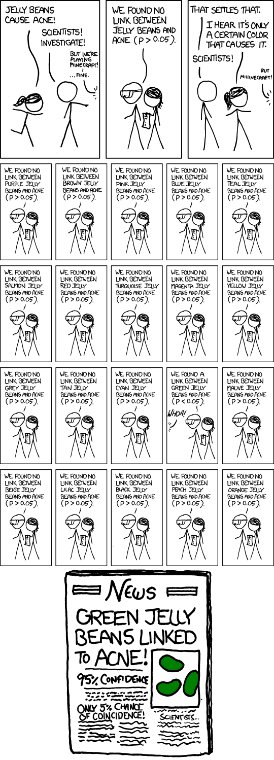
Consider the example from the XKCD comic above. They ran 20 different experiments for different colors of jelly beans, and are looking for signficance at \(p<0.05\).
If we want to control the family-wise error rate at the same level, we simply divide 0.05 by 20! So our new standard for signficance should be \(p<0.0025\).
Bonferroni correction is a good conservative method to control FWER when testing many hypotheses.