Markov Chains
Contents
Markov Chains#
Today we will talk about Markov Chains. Markov chains form a fundamental building block for both the Markov Chain Monte Carlo (MCMC) method and the Hidden Markov Models (HMMs) that will be discussed in the next two weeks.
Consider the following model for the weather in Boston:
If today is sunny, tomorrow will be sunny with probability 0.8; otherwise it will be rainy. If today is rainy, tomorrow will be rainy with probabililty 0.6; otherwise it will be sunny.
We can draw this scenario with a diagram like this:

Why is this useful? It helps us reason about what might happen many days in the future.
For example, we can ask “what is the probability that if today is sunny, tomorrow is sunny and the day after this is rainy” by imaging taking a walk along this graph following the arrows, and multiplying the probability each time.
The great thing is we can do this at the same time for all possible starting conditions for an aribtrary number of days into the future! We’ll do this by combining our knowledge of linear algebra and probability.
This tool is called the Markov Chain after its inventor Andrei Markov, a Russian mathematician working in the late 19th / early 20th century.
Amazingly, we will eventually be able to use Markov chains to help us with the grid search problem we encountered in Bayesian inference, but it will take some background to get there.
A Markov chain is a model of a system that evolves in time. For our purposes we will assume time is discrete, meaning that the system evolves in steps that can be denoted with integers.
At any given time, the Markov chain is in a particular state. The concept of a state is very flexible. We can use the idea of state to represent a lot of things: maybe a location in space, or a color, or a number of people in a room, or a particular value of a parameter. Anything that can be modeled as a discrete thing can be a state.
The basic idea of a Markov chain is that it moves from state to state probabilistically. In any state, there are certain probabilities of moving to each of the other states.
Definitions#
We will denote the state that the Markov chain is in at time \(n\) as \(X_n\). Since the Markov chain evolves probabilistically, \(X_n\) is a random variable.
A defining aspect of a Markov chain is that each time it moves from the current state to the new state, the probability of that transition only depends on the current state.
This is called the Markov property.
The point is that whatever states the chain was in previously do not matter for determining where it goes next. Only the current state affects where the chain goes next.
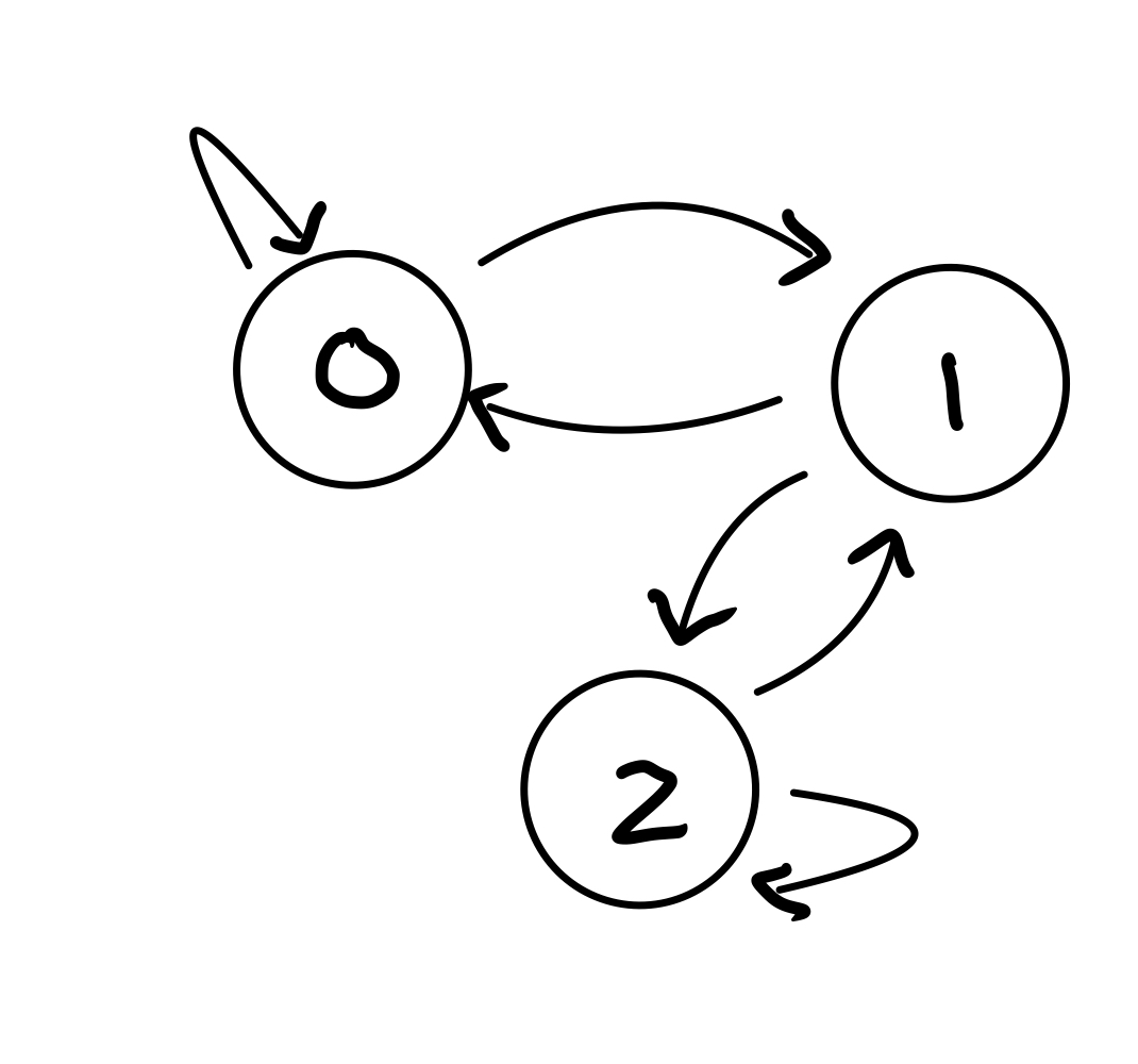
Here is an abstract view of the situation at a particular node 0.
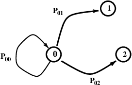
From state 0, on the next step the chain can go to state 1, state 2, or even back to state 0. There is a probability associated with each transition.
Note that the probabilities must sum to 1 – on each transition, the chain must go somewhere (even if it remains at the current node).
Definition. Given a finite set of states \(S = \{1, 2, \dots \}\), a process \(X_0, X_1, \dots\) is a Markov chain on \(S\) if, when the process is in state \(j\), the probability that its next state is \(i\) depends only on \(j\).
Formally, we say that
This the formal statement of the Markov property.
It is usually convenient to work with Markov chains using linear algebra. For that, we use this notation:
Definition. The transition matrix of the chain is the matrix \(P\) with \(P_{ij} = P(X_{n+1} = i \,\vert\, X_{n} = j).\)
Note that by the axioms of probability, for any \(j\):
Hence, the columns of \(P\) each sum to 1. Such a matrix is called a stochastic (or column-stochatic) matrix.
Example 1. Let’s go back to our weather in Boston example
We can see that if at time \(t=0\) the chain is in the “sunny” state, at time \(t=1\) it will either be in a “sunny” state (with probability 0.8) or “rainy” state (with probability 0.2).
This chain has transition matrix:
We can confirm that this is a stochastic matrix by observing that the columns sum to 1.
Example 2. Looking at a bigger, more abstract example, consider the Markov chain below, with states \(\{0, 1, 2, 3\}\) and transition probabilities marked.
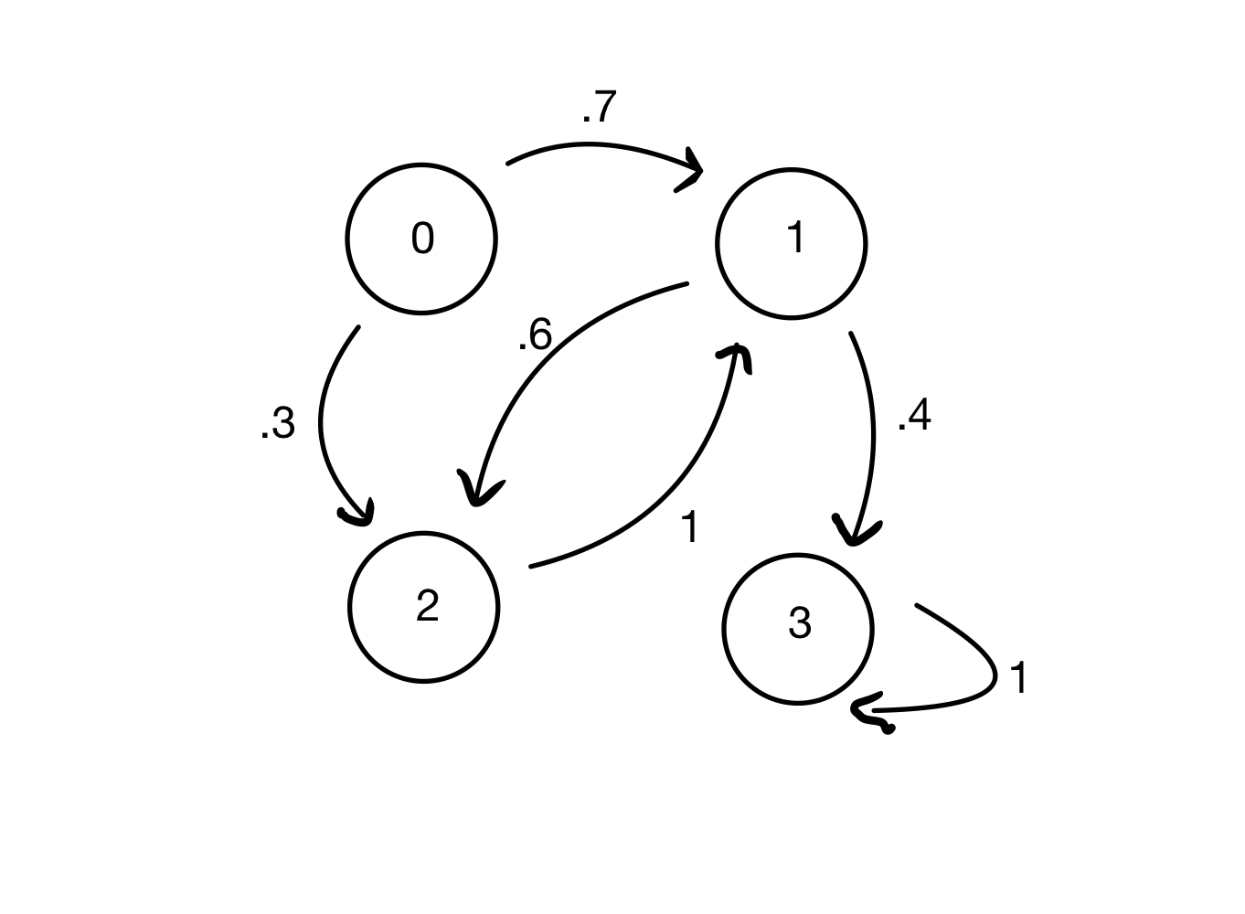
We can see that if at time \(t= 0\) the chain is in state 1, at time \(t = 1\) it will either be in state 2 (with probability 0.6) or state 3 (with probability 0.4).
This chain has transition matrix:
Again, we can confirm that this is a stochastic matrix by summing the columns.
Future States#
OK, so we know that if the chain is in state \(j\), the probability that it will be in state \(i\) at the next step is \(P_{ij}\).
What is the probability it will be in state \(i\) in two steps? three steps? \(n\) steps?
Let’s define the \(n\)-step transition probability matrix \(P^{(n)}\) as
How can we compute \(P^{(n)}\)?
Let’s compute it for the simple case of \(n = 2\):
(This is by the law of total probability.)
which is then:
(By the Markov property)
Now let’s write the expression above in terms of matrices:
Which turns out to be the definition of matrix multiplication.
So $\(P(X_2 = i\,\vert\,X_0 = j) = P^{(2)}_{ij} = P^2_{ij} \)$
In other words, the two-step transition probabilities are given by the square of the \(P\) matrix.
You can see that this generalizes: the \(n\)-step transition probabilities are therefore given by the \(n\)th power of \(P\).
Example 1. Looking at weather in Boston again:
If at time \(t=0\) the chain is in a “sunny” state, at time \(t=2\) it will either be in “sunny” state (with probability 0.72) or a “rainy” state (with probability 0.28).
We can confirm that by computing \(P^2\):
Example 2. And looking at our larger more abstract model again:
If at time \(t= 0\) the chain is in state 1, at time \(t = 2\) it will either be in state 1 (with probability 0.6) or state 3 (with probability 0.4).
We can confirm this by computing \(P^2\):
Distributions Over States#
Now suppose we don’t know with certainty the initial state of the Markov chain, but rather we know a probabiity distribution over the initial states.
We will organize this distribution into a column vector \(\mathbf{x}\). Since it is a distribution, the entries in \(\mathbf{x}\) are nonnegative and sum to 1.
This distribution will evolve in time, so we will denote the distribution at time \(n\) as \(\mathbf{x}_n\).
In other words, \(X_0\) is a random variable with distribution \(P(X_0 = i) = \mathbf{x}_{0,i}\).
Now, we can show that taking one step forward in time corresponds to multiplying \(P\) times \(\mathbf{x}\) as follows:
(by the law of total probability),
so
so
This is called the Forward Kolmogorov Equation. This equation shows how to evolve the probability in time.
It is clear then that
That is, if we know the initial probability distribution at time 0, we can find the distribution at any later time using powers of the matrix \(P\).
Example 1.
If we say that an aribtrary day in Boston has an 80% chance of being sunny, we can calculate whether it will be sunny two days later.
We consider an initial probability distribution over states:
Then to compute the distribution two days later, ie \(\mathbf{x}_2,\) we can use \(P^2\):
Example 2.
Continuing our larger more abstract model again, if we consider an initial probability distribution over states:
Then to compute the distribution two steps later, ie \(\mathbf{x}_2,\) we can use \(P^2\):
Long Term Behavior#
One of the main questions we’ll be asking is concerned with the long run behavior of a Markov Chain.
Let’s consider the long run behavior of Boston weather. We start with just the knowledge that if today is sunny, tomorrow will be sunny with probability 0.8; otherwise it will be rainy. If today is rainy, tomorrow will be rainy with probabililty 0.6; otherwise it will be sunny.
We know we can calculate the probabilty of a sunny day in 2 days or in 10 days, but can we say anything interesting about the weather in 100 or 1,000 days?
Let’s start by writing out the one-step transition matrix for this problem:
Now, let’s assume that day 0 is sunny, and let the chain “run” for a while:
# day 0 is sunny
x = np.array([1, 0])

# P is one-step transition matrix
P = np.array([[0.8, 0.4], [0.2, 0.6]])

for i in range(10):
    print (f'On day {i}, state is {x}')
    x = P @ x
On day 0, state is [1 0]
On day 1, state is [0.8 0.2]
On day 2, state is [0.72 0.28]
On day 3, state is [0.688 0.312]
On day 4, state is [0.6752 0.3248]
On day 5, state is [0.67008 0.32992]
On day 6, state is [0.668032 0.331968]
On day 7, state is [0.6672128 0.3327872]
On day 8, state is [0.66688512 0.33311488]
On day 9, state is [0.66675405 0.33324595]
This seems to be converging to a particular vector: \(\begin{bmatrix} 2/3 \\ 1/3 \end{bmatrix}\).
What if instead, the chain starts from a rainy day?
# day 0 is rainy
x = np.array([0, 1])

# P is one-step transition matrix
P = np.array([[0.8, 0.4], [0.2, 0.6]])

for i in range(10):
    print (f'On day {i}, state is {x}')
    x = P @ x
On day 0, state is [0 1]
On day 1, state is [0.4 0.6]
On day 2, state is [0.56 0.44]
On day 3, state is [0.624 0.376]
On day 4, state is [0.6496 0.3504]
On day 5, state is [0.65984 0.34016]
On day 6, state is [0.663936 0.336064]
On day 7, state is [0.6655744 0.3344256]
On day 8, state is [0.66622976 0.33377024]
On day 9, state is [0.6664919 0.3335081]
Here too, the chain seems to be converging to the same vector \(\begin{bmatrix} 2/3 \\ 1/3 \end{bmatrix}\). This suggests that \(\begin{bmatrix} 2/3 \\ 1/3 \end{bmatrix}\) is a special vector.
Indeed, we can see that if the chain ever exactly reached this vector, it would never deviate after that, because
A vector \(\mathbf{x}\) for which \(P \mathbf{x} = \mathbf{x}\) is called a steady state of the Markov chain \(P\).
Example. If the Markov chain below is in state \(\begin{bmatrix}\frac{6}{11}\\\frac{3}{11}\\\frac{2}{11}\end{bmatrix}\), is it in a steady state?
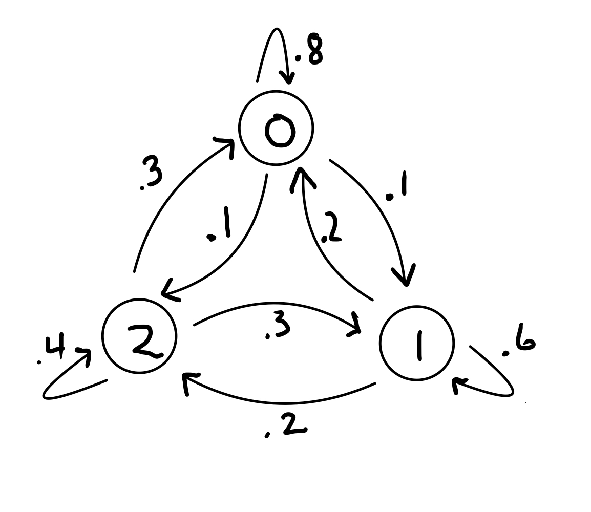
The transition matrix \(P=\begin{bmatrix}0.8&0.2&0.3\\0.1&0.6&0.3\\0.1&0.2&0.4\end{bmatrix}\) and the state \(x=\begin{bmatrix}\frac{6}{11}\\\frac{3}{11}\\\frac{2}{11}\end{bmatrix}\)
We just need to check if \(Px=x\)
$\(\begin{bmatrix}0.8&0.2&0.3\\0.1&0.6&0.3\\0.1&0.2&0.4\end{bmatrix} \begin{bmatrix}\frac{6}{11}\\\frac{3}{11}\\\frac{2}{11}\end{bmatrix}= \begin{bmatrix}\frac{6}{11}\\\frac{3}{11}\\\frac{2}{11}\end{bmatrix}\)$.
So yes, the chain is in a steady state.
Convergence to Steady-State#
So, two remarkable things are happening in the example above:
There is a steady-state vector \(\mathbf{x}\) such that \(P\mathbf{x} = \mathbf{x}\).
It seems that the chain converges to this steady-state, no matter what the starting point is.
These properties are a very interesting and useful behavior, because it means we can talk about the long term behavior of the Markov Chain without worrying about what state the chain started in.
In particular this will turn out to be hugely useful for problems in Bayesian statistics (which we will return to in the next lecture).
So we would very much like to know
When does P have a steady-state?
When can we be sure that P converges to that steady state?
To answer these questions we’ll use a little bit of linear algebra and some ideas from the study of graphs.
First, recall that when a square matrix \(A\) has a nonzero vector \(\mathbf{x}\) such that
for some scalar value \(\lambda\), then we say that \(\mathbf{x}\) is an eigenvector of \(A\), and \(\lambda\) is its associated eigenvalue.
Now \(P\) has two special properties:
None of its entries are negative
Its columns sum to 1
Because of these two properties, we can prove that the largest eigenvalue \(\lambda\) of \(P\) is 1.
This is not hard to prove (and would be proved in a linear algebra course) but we’ll not prove it here. The key to proving it is based on the fact that the columns of \(P\) sum to 1.
For \(\lambda=1\) we see that \( A\mathbf{x} = \mathbf{x} \) making \(x\) a steady state.
This means that every Markov chain has at least one steady-state.
OK, so next we’d like to establish whether the chain has a unique steady-state, that is, does it have only one steady-state?
Definition. We say that a stochastic matrix \(P\) is regular if some matrix power \(P^k\) contains only strictly positive entries.
For
We note that \(P\) does not have every entry strictly positive.
However:
Since every entry in \(P^2\) is positive, \(P\) is a regular stochastic matrix.
Theorem. If \(P\) is an \(n\times n\) regular stochastic matrix, then \(P\) has a unique steady-state vector \({\bf q}.\) Further, if \({\bf x_0}\) is any initial state and \({\bf x_{k+1}} = P{\bf x_k}\) for \(k = 0, 1, 2,\dots,\) then the Markov Chain \(\{{\bf x_k}\}\) converges to \({\bf q}\) as \(k \rightarrow \infty.\)
Note the phrase “any initial state.”
This is a remarkable property of a Markov Chain: it converges to its steady-state vector no matter what state the chain starts in.
We say that the long-term behavior of the chain has “no memory of the starting state.”
Example. In the following chain, for each node, all transitions out of that node are equally probable. So for a node with 2 outgoing transitions, the probabilities are each 1/2. Is this chain a regular Markov Chain?
First, is it a Markov chain?
We need to check if the columns add up to 1.
Second, does it have at least one steady state?
Yes, all Markov chains have at least one steady state.
Third, does it have exactly one steady state?
We need to check if our Markov chain \(P\) has some power \(k\) such that all entries in \(P^k\) are positive.
Let’s check \(k=2\) first:
We already see only positive entries in \(P^2\) so the Markov chain convereges.
Therefore, our example is indeed a regular Markov chain.
Detailed Balance#
Finally, we need to define a special case in which we always know that a Markov chain is in steady-state.
Consider an \(n\)-state Markov chain \(P\), and a steady-state distribution of \(P\) which we’ll denote \(\pi\). So we know that \(P\pi = \pi.\)
In addition to being in steady-state, we say that the chain also satisfies detailed balance with respect to \(\pi\) if
There are \(n^2\) of these equations, and they are called the detailed balance equations.
What do the detailed balance equations represent?
Suppose we start the chain in the stationary distribution, so that \(X_0 \sim \pi.\) Then the quantity \(\pi_i P_{ji}\) represents the “amount” of probability that flows down edge \(i \rightarrow j\) in one time step.
If the detailed balance equations hold, then the amount of probability flowing from \(i\) to \(j\) equals the amount that flows from \(j\) to \(i\). Therefore there is no net flux of probability along the edge \(i \leftrightarrow j\).
Note that it is impossible to have detailed balance if there is only one-way flow between a pair of nodes. If \(P_{ij} = 0\) but \(P_{ji} \neq 0\), then detailed balance is impossible.
A good analogy comes from thinking about traffic flow in New York city and surroundings: let each borough or suburb be represented by a node of the Markov chain, and join two nodes if there is a bridge or tunnel connecting the boroughs, or if there is a road going directly from one to the other. For example, the node corresponding to Manhattan would be connected to Jersey City (via the Holland tunnel) and to Fort Lee (via the George Washington Bridge), etc.
Suppose that cars driving around represent little elements of probability. The city would be in the steady-state distribution if the number of cars in Manhattan, and in all other nodes, doesn’t change with time. This is possible even when cars are constantly driving around in circles, such as if all cars leave Manhattan across the Holland tunnel, drive up to Fort Lee, and enter Manhattan via the George Washington bridge. As long as the total number of cars in Manhattan doesn’t change, the city is in steady-state.
The condition of detailed balance, however, is more restrictive. It says that the number of cars that leaves each bridge or tunnel per unit time equals the number that enter that same bridge or tunnel. For example, the rate at which cars leave Manhattan via the Holland tunnel must equal the rate at which cars enter Manhattan via the Holland tunnel.
Example. We have shown that if the following Markov chain is in state \( \begin{bmatrix}\frac{6}{11}\\\frac{3}{11}\\\frac{2}{11}\end{bmatrix}\), it is in a steady state. However, is it in detalied balance?
To check if it is in detailed balance, we need to confirm that: \(\pi_i P_{ji} = \pi_j P_{ij}\) for all \(i\), \(j\) for:
\(P = \begin{bmatrix}0.8&0.2&0.3\\0.1&0.6&0.3\\0.1&0.2&0.4\end{bmatrix}\) and \( \pi = \begin{bmatrix}\frac{6}{11}\\\frac{3}{11}\\\frac{2}{11}\end{bmatrix}\)
First, note that we don’t need to check cases where \(i=j\) (e.g. \(i=1\) and \(j=1\) in which case the detailed balance equation is \( \pi_1 P_{1,1} = \pi_1 P_{1,1}\) which is true no matter what the numbers are). So let’s start with \(i=1\) and \(j=2\)
Yes! And note we don’t need to check \(i=2,j=1\) because the resulting equation is equivalent to the equation for \(i=1,j=2\)). So we only need to check the other non-redundant pairs of values of i and j: \(i=1,j=3\) and \(i=2,j=3\)
So our Markov chain is in detailed balance.
While not every Markov chain that is in a steady state is in detailed balance, if a system is in detailed balance, it is in steady-state. Intuitively, there is no pair of nodes in the Markov chain that are causing a change in their states.
More formally, consider a system in detailed balance so that \( \pi_i P_{ji} = \pi_j P_{ij}\). Then, for any \(i\):
So \(P\pi = \pi\) and the chain is in steady-state.