Model Fitting

This section draws from Chapter 5 of Deep Learning by Goodfellow, Bengio, and Courville.

Today we will talk about model fitting, likelihood, and log-likelihood functions. This lecture provides a foundation for our next lecture, where we will discuss maximum likelihood estimation.

Model Fitting

The notion of parameter estimation is closely related to the concept called model fitting. We have actually been doing this quite a bit already, but now we want to treat the notion more directly.

Imagine that you know that data is drawn from a particular kind of distribution, but you don’t know the value(s) of the distribution’s parameter(s).

The following table shows a number of common distributions and their corresponding parameters:

Distribution	Parameters \(\theta\)
Bernoulli	\(p\)
Binomial	\((N,p)\)
Poisson	\(\lambda\)
Geometric	\(p\)
Exponential	\(\lambda\)
Uniform	\((a,b)\)
Normal	\((\mu, \sigma)\)

We formalize the problem as follows. We say that data is drawn from a distribution

\[ p(x; \theta). \]

The way to read this is: the probability of \(x\) under a distribution having parameter(s) \(\theta\).

We call \(p(x; \theta)\) a family of distributions because there is a different distribution for each value of \(\theta\).

The graph below illustrates the probability density functions of several normal distributions (from the same parametric family).

Model fitting is finding the parameters \(\theta\) of the distribution given that we know some data \(x\) and assuming that a certain distribution can describe the population.

Notice that in this context, it is the parameters \(\theta\) that are varying (not the data \(x\)).

When we think of \(p(x; \theta)\) as a function of \(\theta\) (instead of \(x\), say) we call it a likelihood.

This change in terminology is just to emphasize that we are thinking about varying \(\theta\) when we look at the probability \(p(x; \theta)\).

For example, consider the dataset below:

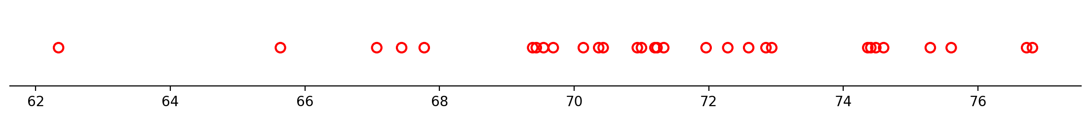
Can you imagine that this dataset might be drawn from a normal distribution?

In that case,

\[ p(x; \theta) = \mathcal{N}(x; \mu, \sigma^2). \]

Then model fitting would consist of finding the \(\mu\) and \(\sigma\) that best match the given data \(x\) shown above.

In other words, the likelihood function gives the probability of observing the given data as a function of the parameter(s). Therefore, the parameters can be estimated by maximizing the likelihood function. We will do that in the next lecture. In this lecture we focus on computing the likelihood function.

Calculating Likelihood

Let’s think about how to calculate likelihood. Consider a set of \(m\) data items

\[ X_s = (x_1, x_2, \dots, x_m) \]

drawn independently from the true but unknown data-generating distribution \(p_{\text{data}}(x)\).

Let \(p_{\text{model}}(x; \theta)\) be a family of probability distributions over the same space.

Then, for any value of \(\theta\), \(p_{\text{model}}(x; \theta)\) maps a particular data item \(x\) to a real number that we can use as an estimate of the true probability \(p_{\text{data}}(x)\).

What is the probability of the entire dataset \(X_s\) under the model?

We assume that the \(x_i\) are independent; so the probabilities multiply.

Therefore, the joint probability is

\[ p_{\text{model}}(X_s; \theta) = p_{\text{model}}(x_1; \theta) \cdot p_{\text{model}}(x_2; \theta) \cdot \ldots \cdot p_{\text{model}}(x_m; \theta). \]

We can use a special shorthand notation to represent products. Just like \(\sum\) is shorthand for summing, \(\prod\) is shortand for taking the product.

For example, the product of two numbers \(a_1\) and \(a_2\) (i.e., \(a_1 a_2\)), can be written as \(\prod_{i=1}^2 a_i\).

So the joint probability can be written as:

\[ p_{\text{model}}(X_s; \theta) = \prod_{i=1}^m p_{\text{model}}(x_i; \theta). \]

Now, each individual \(p_{\text{model}}(x_i; \theta)\) is a value between 0 and 1.

And there are \(m\) of these numbers being multiplied. So for any reasonable-sized dataset, the joint probability is going to be very small.

For example, if a typical probability is \(1/10\), and there are 500 data items, then the joint probability will be a number on the order of \(10^{-500}\).

So the probability of a given dataset as a number will usually be too small to even represent in a computer using standard floating point!

Log-Likelihood

Luckily, there is an excellent way to handle this problem. Instead of using likelihood, we will use the log of likelihood.

The table below shows some of the properties of the natural logarithm.

Product rule	\(\log ab = \log a + \log b\)
Quotient rule	\(\log \frac{a}{b} = \log a - \log b\)
Power rule	\(\log a^n = n \log a\)
Exponential\logarithmic	\(\log e^x = e^{\log x} = x\)

In the next lecture we will see that we are only interested in the maxima of the likelihood function. Since the log function does not change those points (the log is a monotonic function), using the log of the likelihood works for us.

So we will work with the log-likelihood:

\[ \log p_{\text{model}}(X_s; \theta). \]

Which becomes:

\[ \log p_{\text{model}}(X_s; \theta) = \log \prod_{i=1}^m p_{\text{model}}(x_i; \theta) = \sum_{i=1}^m \log p_{\text{model}}(x_i; \theta). \]

This way we are no longer multiplying many small numbers, and we work with values that are easy to represent.

Note: The log of a number less than one is negative, so log-likelihoods are always negative values.

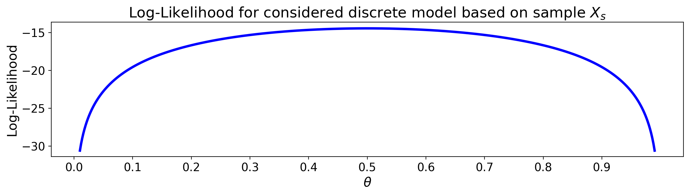
Example.

Suppose that \(X\) is a discrete random variable with the probability mass function shown below.

\(x\)	\(0\)	\(1\)	\(2\)	\(3\)
\(p(x;\theta)\)	\(\frac{2}{3}\theta\)	\(\frac{1}{3}\theta\)	\(\frac{2}{3}\left(1-\theta\right)\)	\(\frac{1}{3}\left(1-\theta\right)\)

Here \(0\leq \theta \leq 1\) is a parameter. The following 10 independent observations were taken from this distribution:

\[X_s = (3,0,2,1,3,2,1,0,2,1).\]

We want to find the corresponding log-likelihood function.

Based on the observed data sample, the (joint) likelihood function is equal to

\[p(X_s;\theta) = \prod_{i=1}^{10} p\left(x^{(i)}; \theta\right)=p(0;\theta)^2p(1;\theta)^3p(2;\theta)^3p(3;\theta)^2\]

\[=\left( \frac{2}{3}\theta \right)^2 \left( \frac{1}{3}\theta \right)^3 \left(\frac{2}{3}\left(1-\theta\right)\right)^3 \left(\frac{1}{3}\left(1-\theta\right)\right)^2.\]

Since the likelihood function is given by

\[ p(X_s;\theta) = \left( \frac{2}{3}\theta \right)^2 \left( \frac{1}{3}\theta \right)^3 \left(\frac{2}{3}\left(1-\theta\right)\right)^3 \left(\frac{1}{3}\left(1-\theta\right)\right)^2,\]

the log-likelihood function can be written as

\[\log p(X_s;\theta) = \log \left( \left( \frac{2}{3}\theta \right)^2 \left( \frac{1}{3}\theta \right)^3 \left(\frac{2}{3}\left(1-\theta\right)\right)^3 \left(\frac{1}{3}\left(1-\theta\right)\right)^2 \right) \]

\[ =2\left(\log\frac{2}{3}+ \log \theta \right) + 3\left(\log\frac{1}{3}+ \log \theta \right) + 3\left(\log\frac{2}{3}+ \log (1-\theta) \right) + 2\left(\log\frac{1}{3}+ \log (1-\theta) \right)\]

\[= 5\log \theta + 5\log (1-\theta) + 5\log\frac{2}{9}.\]

We can visualise the log-likelihood function by varying \(\theta\).

Example.

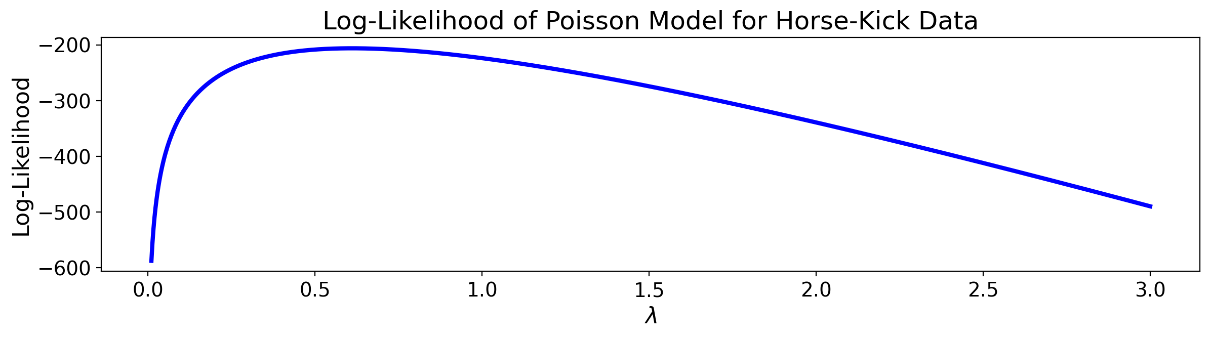
As an example, let’s return to Bortkeiwicz’s horse-kick data, and see how the log-likelihood changes for different values of the Poisson parameter \(\lambda\).

Recall that Bortkeiwicz had collected deaths by horse-kick in the Prussian army over a span of 200 years, and was curious whether they occurred at a constant, fixed rate.

To do this he fitted the data to a Poisson distribution. To do that, he needed to estimate the parameter \(\lambda\).

Let’s see how the log-likelihood of the data varies as a function of \(\lambda\).

Deaths Per Year	Observed Instances
0	109
1	65
2	22
3	3
4	1
5	0
6	0

As a reminder, \(\lambda\) is rate of deaths per year, and \(T = 1\) reflects that we are interested in one-year intervals.

The Poisson distribution predicts:

\[ P[k \mbox{ deaths in time } T] = (\lambda T)^k \frac{e^{- \lambda T}}{k!}\]

Since \(T = 1\) we can drop it, and so the likelihood of a particular number of deaths \(x_i\) in year \(i\) is:

\[ p(x_i; \lambda) = \lambda^{x_i} \frac{e^{- \lambda}}{x_i!}\]

The likelihood function then becomes

\[p(X_s;\lambda) = \prod_{i=1}^{m} \lambda^{x_i} \frac{e^{- \lambda}}{x_i!}.\]

The corresponding log-likelihood function can be written as

\[ \log p(X_s; \lambda) = \log \left(\prod_{i=1}^{m} \lambda^{x_i} \frac{e^{- \lambda}}{x_i!}\right) = \sum_{i=1}^m \log \left(\lambda^{x_i} \frac{e^{- \lambda}}{x_i!}\right). \]

Note that the log-likelihood of a particular number of deaths \(x_i\) in year \(i\) is equal to

\[ \log p(x_i; \lambda) = \log \left(\lambda^{x_i} \frac{e^{- \lambda}}{x_i!}\right) = x_i \log \lambda - \lambda - \log x_i! \]

Using this we can express the log-likelihood of the data as

\[ \log p(X_s; \lambda) = \sum_{i=1}^m \left( x_i \log \lambda - \lambda - \log x_i!\right) \]

Which looks like this as we vary \(\lambda\):

Recall that for an arbitrary Normal distribution with mean \(\mu\) and variance \(\sigma^2\), the PDF is given by

\[ p_{\mu,\sigma}(x) = \frac{1}{\sigma \sqrt{2 \pi}} e^{-\frac{1}{2}\left(\frac{x-\mu}{\sigma}\right)^2}. \]

Francis Galton's "Bean Machine"

Example.

Suppose \(X_s =(x_1, \dots, x_m)\) represents the observed data from a normal distribution \(N(\mu,\sigma^2)\), where \(\mu\) and \(\sigma\) are the unknown parameters. To fit the data to a normal distribution we need to estimate both \(\mu\) and \(\sigma\).

The likelihood function is the product of the marginal densities:

\[p\left(X_s; \mu, \sigma \right) = p\left(x_1, \dots, x_m; \mu, \sigma \right)= \prod_{i=1}^{m}\frac{1}{\sigma \sqrt{2\pi}}e^{-\frac{1}{2}\left(\frac{x_i - \mu}{\sigma} \right)^2}.\]

This can be rewritten as

\[p\left(X_s; \mu, \sigma\right)= \left(\frac{1}{\sigma \sqrt{2\pi}}\right)^m \exp\left(\sum_{i=1}^m -\frac{1}{2}\left(\frac{x_i - \mu}{\sigma} \right)^2 \right).\]

Since the likelihood function is equal to

\[p\left(X_s; \mu, \sigma \right)= \left(\frac{1}{\sigma \sqrt{2\pi}}\right)^m \exp\left(\sum_{i=1}^m -\frac{1}{2}\left(\frac{x_i - \mu}{\sigma} \right)^2 \right),\]

the log likelihood becomes

\[ \log p\left(X_s; \mu, \sigma \right) = \log \left(\sigma \sqrt{2\pi}\right)^{-m} + \sum_{i=1}^m \left(-\frac{1}{2}\right)\left(\frac{x_i - \mu}{\sigma} \right)^2 \]

\[= -m\log \sigma - \frac{m}{2}\log(2\pi) -\frac{1}{2\sigma^2}\sum_{i=1}^m \left(x_i - \mu \right)^2.\]

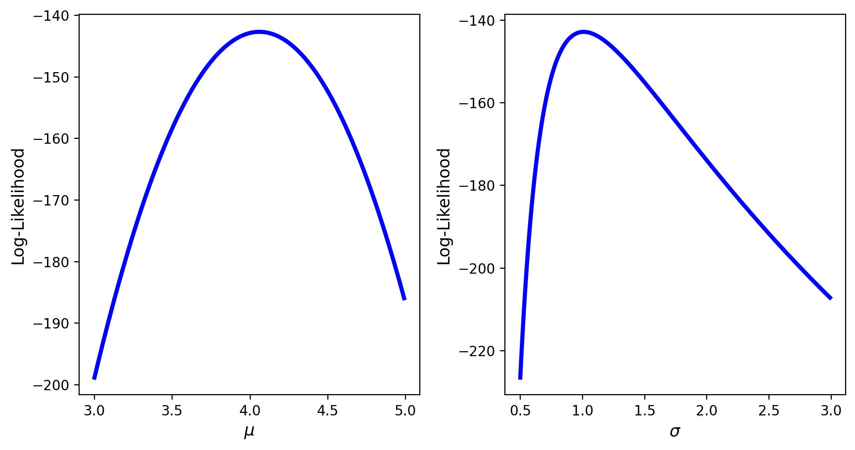
Visualizing Log-Likelihood

We consider a sample of size 100 from a normal distribution. Our goal is to visualize the corresponding log-likelihood function. To do so, first we create the log-likelihood function.

# log-likelihood function for a normal distribution
# input: sample, parameters' domains
def normloglik(X,muV,sigmaV):
    m = len(X)
    return -m/2*np.log(2*np.pi) - m*np.log(sigmaV)\
    - (np.sum(np.square(X))- 2*muV*np.sum(X)+m*muV**2)/(2*sigmaV**2)

Note: The log-likelihood function of the normal distribution can also be written as

\[\log p\left(X_s; \mu, \sigma \right) = - \frac{m}{2}\log(2\pi) -m\log \sigma -\frac{1}{2\sigma^2}\left( \sum_{i=1}^m \left(x_i\right)^2 - 2\mu \sum_{i=1}^m x_i + m\mu^2 \right).\]

If neither of the parameters is known, we can use a surface plot to visualize the log-likelihood as a function of both parameters.

Alternatively, if one of the parameters is known, we visualize the log-likelihood as function of the unknown parameter.