Consistency, Efficiency, Sufficiency

This section draws from Chapter 8 of Mathematical Statistics and Data Analysis by John A. Rice and Probability & Statistics with Applications to Computing by Alex Tsun.

In our first lecture on parameter estimation we introduced a number of criteria that can be used to describe the quality of a parameter. Namely, the bias, the variance, and the mean squared error (MSE). Bias measures whether or not, in expectation, our estimator is equal to the true value of the paramter. MSE measures the expected squared difference between our estimator and the true value of the paramter. If our estimator is unbiased, then the MSE of our estimator is equal to the variance.

Today we will discuss even more desirable properties of estimators.

Consistency

It was mentioned in the previous lectures that both ML and method of moments estimates are consistent. However, we have not given a precise definition of this property yet. Let us look at consistency in more detail.

If we are estimating a scalar quantity, the estimate should improve as we gather more data. Ideally, the estimate should converge to the true value as the number of data items grows large. Estimators that achieve this are said to be consistent.

Definition. Let \(\hat{\theta}_m\) be an estimate of a parameter \(\theta\) based on a sample of size \(m\). Then \(\hat{\theta}_m\) is said to be consistent in probability if \(\hat{\theta}_m\) converges in probability to \(\theta\) as \(m\) approaches infinity. That is, for any \(\varepsilon >0\),

\[P(|\hat{\theta}_m - \theta| > \varepsilon) \to 0 \quad \text{ as } m \to \infty.\]

Example. Recall that if \(x_1, x_2, ..., x_m\) is an i.i.d. sample from the continuous uniform distribution on \((0,\theta)\). Then the method of moments estimate for \(\theta\) is given by

\[\hat{\theta} = \frac{2}{m} \sum_{i=1}^m x_i.\]

Show that \(\hat{\theta}\) is a consistent estimate of \(\theta\).

Solution. To show that \(\hat{\theta}\) is consistent, we need to prove first that \(\hat{\theta}\) is unbiased.

Since the sample is from a continuous uniform distribution on \((0,\theta)\), \(E[x_i] = \frac{\theta}{2}\) for \(1 \leq i \leq m.\) From this we obtain

\[E[\hat{\theta}] = E\left[ \frac{2}{m} \sum_{i=1}^m x_i \right] = \frac{2}{m} \sum_{i=1}^m E[x_i] = \frac{2}{m} m \frac{\theta}{2} = \theta.\]

Hence, the estimate is indeed unbiased.

Since \(\hat{\theta}\) is unbiased, we have that

\[P(|\hat{\theta} - \theta| > \varepsilon) = P(\left|\hat{\theta} - E[\hat{\theta}]\right| > \varepsilon).\]

Now, we can apply Chebyshev’s inequality:

\[P(\left|\hat{\theta} - E[\hat{\theta}]\right| > \varepsilon) \leq \frac{\operatorname{Var}{\hat{\theta}}}{\varepsilon^2}.\]

Substituting the expression for \(\hat{\theta}\) in the variance gives us the following:

\[\begin{align*} P(\left|\hat{\theta} - E[\hat{\theta}]\right| > \varepsilon) & \leq \frac{\operatorname{Var}{\hat{\theta}}}{\varepsilon^2} \\ & = \frac{\operatorname{Var}\left( \frac{2}{m} \sum_{i=1}^m x_i\right)}{\varepsilon^2} \\ & = \frac{\frac{4}{m^2} \operatorname{Var}\left( \sum_{i=1}^m x_i\right)}{\varepsilon^2}\\ & = \frac{\frac{4}{m^2} m \operatorname{Var}(x_i)}{\varepsilon^2} \\ & = \frac{4 \operatorname{Var}(x_i)}{m \varepsilon^2}. \end{align*}\]

It remains to take the limit with the above expression.

\[\lim_{m \to \infty} P(|\hat{\theta} - \theta| > \varepsilon) \leq \lim_{m \to \infty} \frac{4 \operatorname{Var}(x_i)}{m \varepsilon^2} = 0.\]

This implies that \(\hat{\theta}\) is a consistent estimate of \(\theta\).

Consistency vs Unbiasedness

Based on the above description you might be wondering whether consistency is the same as unbiasedness. It is not. There is a subtle difference between consistency and unbiasedness.

For instance, we have just shown that our estimator \(\hat{\theta} = \frac{2}{m} \sum_{i=1}^m x_i\) for the continuous uniform distribution on \((0,\theta)\) is both unbiased and consistent. As we saw in the above example, the second property follows from the fact that its variance goes to zero as the sample size approaches infinity.

On the other hand, we can easily construct an estimator that is unbiased but not consistent for the same i.i.d. sample from the continuous distribution on \((0,\theta)\). If you just take the first realization and multiply it by 2, ignoring all other realizations, the estimator becomes \(\hat{\beta} = 2x_1\).

Clearly, the \(\hat{\beta}\) is unbiased: $\(\operatorname{bias}(\hat{\beta}) = E\left[\hat{\beta}\right] - \theta = 2E[x_1] - \theta = 2\frac{\theta}{2}- \theta = 0.\)$

Since our estimator does not use all \(m\) data points, the estimate does not improve with a higher value of \(m\). Hence, \(\hat{\beta}\) is not consistent.

Efficiency

So far we have learned how to compute the ML estimates and the method of moments estimates. In the future, we will introduce the Bayesian approach to parameter estimation. We also said that, in general, any function of the data qualifies as an estimator.

Given this variety of possible parameter estimates, how would we choose which one to use?

Qualitatively, it would be sensible to choose the estimate whose sampling distribution was most highly concentrated about the true parameter value.

This implies that we need to specify a quantitative measure of such concentration. Fortunately, we have already defined it. The mean squared error, MSE, is the most commonly used measure of concentration.

Recall that the MSE of \(\hat{\theta}\) is simply equal to

\[\begin{align*} \operatorname{MSE}\left(\hat{\theta}\right) & = E\left[\left(\hat{\theta} - \theta\right)^2\right] \\ & = \operatorname{bias}\left(\hat{\theta}\right)^2 + \operatorname{Var}\left(\hat{\theta}\right). \end{align*}\]

If the estimate \(\hat{\theta}\) is unbiased, \(\operatorname{MSE}\left(\hat{\theta}\right) = \operatorname{Var}\left(\hat{\theta}\right)\).

Therefore, if we are considering two unbiased estimates, then comparison of their mean squared errors reduces to comparison of their variances.

Definition. Given two estimates, \(\hat{\theta}\) and \(\hat{\beta}\), of a parameter \(\theta\), the efficiency of \(\hat{\theta}\) relative to \(\hat{\beta}\) is defined as

\[\operatorname{eff}(\hat{\theta},\hat{\beta}) = \frac{\operatorname{Var}(\hat{\beta})}{\operatorname{Var}(\hat{\theta})}.\]

Thus, if the efficiency is smaller than 1, \(\hat{\theta}\) has a larger variance than \(\hat{\beta}\) has. In this case, \(\hat{\theta}\) is less efficient than \(\hat{\beta}\).

This comparison is most meaningful when both \(\hat{\theta}\) and \(\hat{\beta}\) are unbiased or when both have the same bias.

Based on the above discussion it becomes obvious that it would be great if the MSE of an estimate was as low as possible. Hence, we might ask whether there is a lower bound for the MSE of any estimate.

If such a lower bound exists, it should function as a benchmark against which estimates could be compared. Suppose that an estimate achieved this lower bound, then we know that its MSE cannot be improved upon.

When the estimate is unbiased, the Cramér-Rao inequality, also known as the information inequality, provides such a lower bound.

Fisher Information

Before we present the Cramér-Rao inequalit, we need to define a measure for the amount of information that a sample of data contains about the unknown parameter, the so-called Fisher information. This concept was introduced by Ronald Fisher.

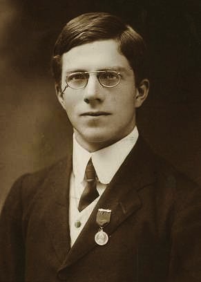
Ronald Fisher

Definition. Let \(\theta\) be a parameter or a vector of parameters. Assume that the probability mass function (or probability density function) of \(X\) depends on \(\theta\). Furthermore, let \(X_s = (x_1, x_2, ..., x_m)\) be i.i.d. sample from probability mass function (or probability density function) of \(X\). Then Fisher information of \(\theta\) is defined as

\[I(\theta) = E\left[ \left( \frac{\partial \log p(X_s; \theta) }{\partial \theta} \right)^2 \right] = - E\left[ \frac{\partial^2 \log p(X_s; \theta) }{\partial \theta^2} \right],\]

where \(p(X_s; \theta)\) denotes the likelihood of the data given \(\theta\).

The above definition is definitely a mouthful, but it includes the concepts that we are already familiar with and know how to compute. Namely, the likelihood and the log-likelihood.

Recall that we can take the second derivative of the log-likelihood to confirm that our MLE is indeed a maximizer. To obtain the Fisher information all we have to do is take the expectation of this second derivative.

Cramér-Rao Inequality

The Cramér-Rao inequality was developed independently by H. Cramér and C.R. Rao during the 1940s.

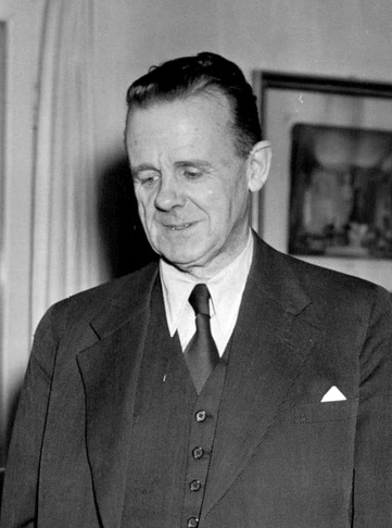
Harald Cramér

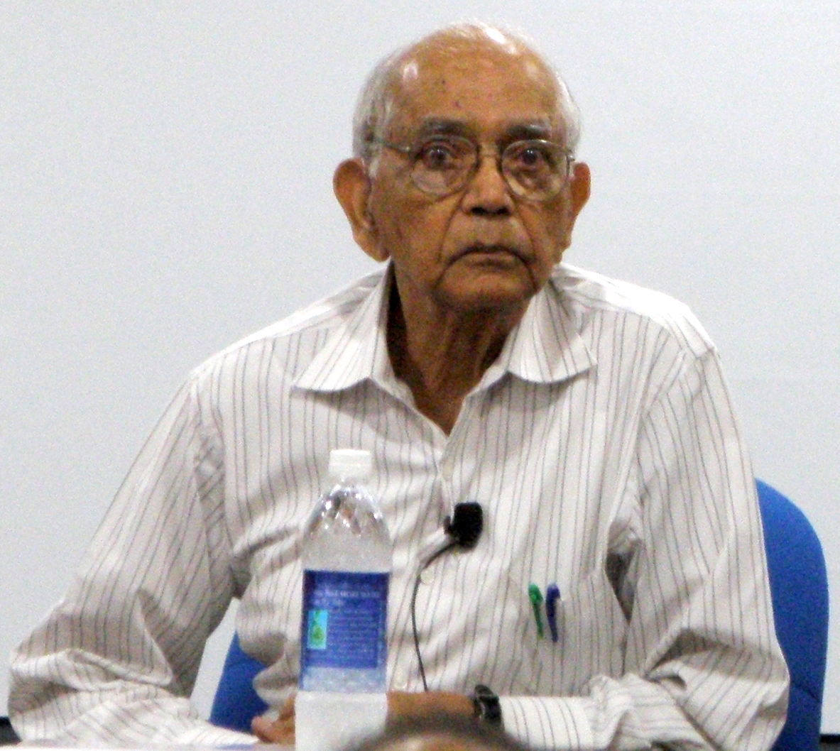
Calyampudi Radhakrishna Rao

Theorem. Let \(\theta\) be a parameter or a vector of parameters. Assume that the probability mass function (or probability density function) of \(X\) depends on \(\theta\). Furthermore, let \(X_s = (x_1, x_2, ..., x_m)\) be i.i.d. sample from probability mass function (or probability density function) of \(X\). If \(\hat{\theta}\) is an unbiased estimate of \(\theta\), then

\[\operatorname{Var}(\hat{\theta}) \geq \frac{1}{I(\theta)}.\]

Proof. The proof of this theorem is outside the scope of this class. An interested reader can consult, for instance, Mathematical Statistics and Data Analysis by John A. Rice.

The Cramér-Rao inequality gives a lower bound on the variance of any unbiased estimate. This bound is equal to \(\frac{1}{I(\theta)}\) and is called the Cramér-Rao lower bound.

Definition. An unbiased estimate whose variance achieves the Cramér-Rao lower bound is called efficient.

Efficiency is another highly desirable property of estimators.

Example. Let \(x_1, x_2, ..., x_m\) is an i.i.d. sample from the Poisson distribution with parameter \(\theta\). An estimate for \(\theta\) is given by

\[\hat{\theta} = \frac{1}{m} \sum_{i=1}^m x_i.\]

Show that \(\hat{\theta}\) is an efficient estimate of \(\theta\).

Note: this estimate can be computed using either the maximum likelihood estimation or the method of moments estimation.

Solution. To show that an estimate is efficient we need to show that it is unbiased and that its variance achieves the Cramér-Rao lower bound.

Let us start with the first requirement, the unbiasedness.

\[E[\hat{\theta}] = E\left[ \frac{1}{m} \sum_{i=1}^m x_i \right] = \frac{1}{m} \sum_{i=1}^m E[x_i] = \frac{1}{m} m \theta = \theta.\]

Thus, the estimate is indeed unbiased. Here, we used the fact that the mean of the Poisson distribution with parameter \(\theta\) is equal to \(\theta\).

Next, we need to compute the variance of \(\hat{\theta}\) and check whether it is equal to \(\frac{1}{I(\theta)}\).

Using the fact that the sample is i.i.d. and that for the Poisson distribution with paramter \(\theta\) the variance is equal to \(\theta\), we obtain:

\[\operatorname{Var}(\hat{\theta}) = \operatorname{Var}\left( \frac{1}{m} \sum_{i=1}^m x_i \right) = \frac{1}{m^2} \sum_{i=1}^m \operatorname{Var}(x_i) = \frac{1}{m^2}m \theta = \frac{\theta }{m}.\]

It remains to compute the Cramér-Rao lower bound.

In the lecture on MLE we derived an expression for the first derivative of the log-likelihood function for the Poisson distribution:

\[ \frac{\partial}{\partial\theta}\log p(X_s; \theta) = \frac{1}{\theta} \sum_{i=0}^m x_i - m.\]

Thus, to calculate the second derivative w.r.t. \(\theta\) we simply differentiate the above result.

\[ \frac{\partial^2}{\partial\theta^2}\log p(X_s; \theta) = \frac{\partial^2}{\partial\theta^2} \left( \frac{1}{\theta} \sum_{i=0}^m x_i - m \right) = -\frac{1}{\theta^2} \sum_{i=0}^m x_i.\]

The expected value of the above expression is given by

\[E\left[\frac{\partial^2}{\partial\theta^2}\log p(X_s; \theta)\right] = E\left[ -\frac{1}{\theta^2} \sum_{i=0}^m x_i \right] = -\frac{1}{\theta^2} \sum_{i=0}^m E[x_i] = -\frac{1}{\theta^2} m \theta = -\frac{m}{\theta}.\]

Hence, Fisher information is equal to

\[I(\theta) = -E\left[\frac{\partial^2}{\partial\theta^2}\log p(X_s; \theta)\right] = \frac{m}{\theta}.\]

From which we obtain the Cramér-Rao lower bound:

\[\frac{1}{I(\theta)} = \frac{\theta}{m}.\]

The bound is equal to the variance that we computed before: $\(\operatorname{Var}(\hat{\theta}) = \frac{\theta}{m} = \frac{1}{I(\theta)}.\)$

Since \(\hat{\theta}\) is unbiased and its variance achieves the Cramér-Rao lower bound, we conclude that the estimate is efficient.

Bonus material:

Sufficiency

The final property of a paramter estimate that we are going to consider is sufficiency. Just like we want our estimates to be consistent and efficient, we also want them to be sufficient.

To explain the concept of sufficiency we will consider the following situation. Suppose we have i.i.d. realizations \(X_s = (x_1, \dots, x_m)\) from a known distribution with unknown parameter \(\theta\). Imagine we have two statisticians:

• Statistician \(Y\): They know the entire sample \(X_s = (x_1, \dots, x_m)\), all \(m\) data points.

• Statistician \(Z\): They only know \(T(x_1, \dots, x_m) = t\), a single number which is a function of the realizations. For example, the sample mean.

If Statistician \(Z\) can do just as good a job as Statistician \(Y\), given “less information”, then \(T(x_1, \dots, x_m)\) is a sufficient statistic.

For instance, consider a sequence of independent Bernoulli trials with unknown probability of success, \(\theta\). Our intuition tells us that the total number of successes contains all the information about \(\theta\) that there is in the sample. The order in which the successes occurred, for example, does not give any additional information. The following definition formalizes this idea.

Definition. A statistic \(T(X_1,..., X_n)\) is said to be sufficient for \(\theta\) if the conditional distribution of \(X_1,..., X_n\), given \(T = t\) and \(\theta\) does not depend on \(\theta\):

\[P(X_1=x_1,..., X_n=x_n | T=t, \theta) = P(X_1=x_1,..., X_n=x_n | T=t).\]

In other words, given the value of a sufficient statistic \(T\), we can gain no more knowledge about \(\theta\) from knowing more about the probability distribution of \(X_1,..., X_n\).

Note: All estimators can be viewed as statistics because they take in our \(m\) data points and produce a single number, so the above definition is relevant for estimators.

Neyman-Fisher Factorization Criterion

The provided definition is hard to check, but it turns out that there is a criterion that helps us determine whether an estimator is sufficient.

Theorem. A necessary and sufficient condition for \(T(X_1,..., X_m)\) to be sufficient for a parameter \(\theta\) is that the joint probability function (density function \(f\) or frequency function \(p\)) factors in the form

\[p(x_1,...,x_m|\theta) = g[T(x_1,...,x_m),θ]h(x_1,...,x_m).\]

Proof. The proof of this theorem is outside the scope of this class. An interested reader can consult, for instance, Mathematical Statistics and Data Analysis by John A. Rice.

The theorem tells us that we need to split the joint probability function into a product of two terms:

• For the first term \(g\), you can only know the sufficient statistic (single number) \(T(x_1, ... , x_n)\) and \(\theta\). You may not know each individual realization \(x_i\).

• For the second term \(h\), you are allowed to know each individual realization, but not \(\theta.\)

Example. Let \(x_1, x_2, ..., x_m\) is an i.i.d. sample from the Poisson distribution with parameter \(\theta\). Show that \(T(x_1,..., x_m) = \sum_{i=1}^m x_i\) is a sufficient statistic.

Solution. We take our Poisson probability function and split it into smaller terms:

\[\begin{align*} p(x_1,...,x_n|\theta) &= \prod_{i=1}^m e^{-\theta} \frac{\theta^{x_i}}{x_i!}\\ &= \left(\prod_{i=1}^m e^{-\theta} \right)\left(\prod_{i=1}^m \theta^{x_i} \right) \left(\prod_{i=1}^m \frac{1}{x_i!} \right)\\ &= \frac{e^{m\theta} \theta^{\sum_{i=1}^m x_i}}{\prod_{i=1}^m x_i!}\\ &= e^{m\theta} \theta^{T(x_1,..., x_m)} \frac{1}{\prod_{i=1}^m x_i!}. \end{align*}\]

Set \(g[T(x_1,...,x_m),θ] = e^{m\theta} \theta^{T(x_1,..., x_m)}\) and \(h(x_1,...,x_m) = \frac{1}{\prod_{i=1}^m x_i!}.\)

Then by Neyman-Fisher Factorization Criterion \(T(x_1,..., x_m) = \sum_{i=1}^m x_i\) is a sufficient statistic.

Notice that the mean \(\frac{T(x_1,..., x_m)}{m}\) is sufficient as well. This follows from the fact that knowing the total number of events and the average number of events is equivalent, because we know \(m\).