Limit Theorems

Note

This lecture is based on the material from Section 8 of A First Course in Probability by Sheldon Ross and Chapter 5 of Mathematical Statistics and Data Analysis by John A. Rice.

Today we will discuss limit theorems that describe the limiting behavior of the sum of independent random variables as the number of summands becomes large. Limit theorems are considered to be some of the most important theoretical results in probability theory. They are extremely useful, because many commonly computed statistical quantities, such as averages, can be presented as sums.

Markov’s and Chebyshev’s Inequalities

We mentioned earlier that the variance or standard deviation of a random variable gives an indication as to how spread out its possible values are. Chebyshev’s inequality lends a quantitative aspect to this indication.

To prove the this inequality we first state another important result known as Markov’s inequality.

Markov’s Inequality

Theorem. Let $X$ be a random variable that takes only nonnegative values. Then, for any value $a>0,$

$$P(X\ge a)\le \frac{E[X]}{a}.$$

Proof. The proof is outside the scope of this class. An interested reader can consult, for instance, A First Course in Probability by Sheldon Ross.

The importance of Markov’s inequality is that it enables us to derive bounds on probabilities when only the mean of the probability distribution is known. Of course, if the actual distribution was known, then the desired probabilities could be computed exactly and we would not need to use the inequality.

Chebyshev’s Inequality

Similarly to Markov’s inequality, Chebyshev’s inequality allows us to derive bounds on probabilities. However, it requires both the mean and the variance of the probability distribution to be known.

Theorem. Let $X$ be a random variable with mean $\mu$ and variance ${\sigma }^2$. Then, for any $t>0$,

$$P(|X-\mu |\ge t)\le \frac{{\sigma }^2}{t^2}.$$

Proof. Let $Y=(X-\mu {)}^2$. Then $Y$ is a nonnegative random variable and we can apply Markov’s inequality. Letting $a=t^2$ we obtain

$$P(Y\ge t^2)=P((X-\mu {)}^2\ge t^2)\le \frac{E[(X-\mu {)}^2]}{t^2}=\frac{{\sigma }^2}{t^2}.$$

Since $(X-\mu {)}^2\ge t^2$ if and only if $|X-\mu |\ge t$, the above equation is equivalent to

$$P(|X-\mu |\ge t)\le \frac{{\sigma }^2}{t^2}.$$

The theorem says that if the variance is very small, there is a high probability that $X$ will not deviate much from the mean.

For another interpretation, we can set $t=k\sigma$ so that the inequality becomes $$P(|X-\mu |\ge k\sigma )\le \frac{1}{k^2}.$$

For example, the probability that $X$ is more than $4\sigma$ away from $\mu$ is less than or equal to $\frac{1}{16}.$

As Chebyshev’s inequality is valid for all distributions of the random variable $X$, we cannot expect the bound on the probability to be very close to the actual probability in most cases. For this reason the inequality is typically used as a theoretical tool for proving other results, such as the weak law of large numbers.

The Weak Law of Large Numbers

It is commonly believed that if a fair coin is tossed many times and the proportion of heads is calculated, that proportion will be close to $\frac{1}{2}$.

Mathematician John Kerrich tested this belief empirically while detained as a prisoner during World War II. He tossed a coin 10,000 times and observed heads 5067 times.

The law of large numbers is a mathematical formulation of this belief.

The tosses of the coin are modeled as independent random trials. The random variable $X_i$ takes on the value 0 or 1 according to whether the $i$th trial results in a tail or a head. The proportion of heads in $n$ trials is

$${\bar{X}}_n=\frac{1}{n}\sum _{i=1}^n{X}_i.$$

The law of large numbers states that ${\bar{X}}_n$ approaches $\frac{1}{2}$ in a sense that is specified by the following theorem.

Theorem. Let $X_1,X_2,...,X_i,...$ be a sequence of independent random variables with $E[X_i]=\mu$ and $\mathrm{Var}(X_i)={\sigma }^2$. Let ${\bar{X}}_n=\frac{1}{n}\sum _{i=1}^n{X}_i.$ Then, for any $\epsilon >0$,

$$P(|{\bar{X}}_n-\mu |\ge \epsilon )\to 0\text{ as }n\to \mathrm{\infty }.$$

Proof. We first find $E[{\bar{X}}_n]$ and $\mathrm{Var}({\bar{X}}_n).$

$$E[{\bar{X}}_n]=\frac{1}{n}\sum _{i=1}^{n}E(X_i)=\mu .$$

Since $X_i$’s are independent,

$$\mathrm{Var}({\bar{X}}_n)=\frac{1}{n^2}\sum _{i=1}^n\mathrm{Var}(X_i)=\frac{{\sigma }^2}{n}.$$

From Chebyshev’s inequality follows that

$$P(|{\bar{X}}_n-\mu |\ge \epsilon )\le \frac{\mathrm{Var}({\bar{X}}_n)}{{\epsilon }^2}=\frac{{\sigma }^2}{n{\epsilon }^2}\to 0,\text{ as }n\to \mathrm{\infty }.$$

The above theorem is known as the weak law of large numbers, because ${\bar{X}}_n$ converges in probability to $\mu .$

There is another mode of convergence, called strong convergence, which asserts more than convergence in probability.

Strong convergence implies that, beyond some point in the sequence, the difference between ${\bar{X}}_n$ and $\mu$ is always less than $\epsilon$, but the location of that point is random.

The above result can also be proven and is known as the strong law of large numbers. This version of the law of large numbers is outside the scope of this course.

The Central Limit Theorem

In applications, we often want to find $P(a<X<b)$ or a similar expression without knowing the distribution of $X$ precisely. Sometimes it is possible to achieve this by approximating the distribution of $X$.

The approximation is often arrived at the central limit theorem (CLT). The CLT is the most famous limit theorem in probability theory and is the main topic of today’s lecture.

The CLT is concerned with a limiting property of sums of random variables.

If $X_1,X_2,...$ is a sequence of independent random variables with mean $\mu$ and variance ${\sigma }^2$, and if

$$S_n=\sum _{i=1}^n{X}_i$$

we already know from the weak law of large numbers that $\frac{S_n}{n}$ converges to $\mu$ in probability.

The CLT is concerned not with the fact that the ratio $\frac{S_n}{n}$ converges to $\mu$ but with how it fluctuates around $\mu$.

Theorem. Let $X_1,X_2,...$ be a sequence of independent and identically distributed random variables, each having mean $\mu$ and variance ${\sigma }^2$. Let $S_n=\sum _{i=1}^n{X}_i$. Then

$$\frac{S_n-n\mu }{\sigma \sqrt{n}}$$

tends to the standard normal distribution as $n\to \mathrm{\infty }$.

Proof. The proof is outside the scope of this class. An interested reader can consult, for instance, A First Course in Probability by Sheldon Ross.

There are many central limit theorems of various degrees of abstraction and generality. The above version is one of the simplest versions. Loosely put, the above version tells us the following:

If $X_1,X_2,...,X_n$ are independent random variables with mean $\mu$ and standard deviation $\sigma$, and if $n$ is large, then, $X_1+...+X_n$ is approximately normally distributed with mean $n\mu$ and standard deviation $\sqrt{n}\sigma$.

Another relatively simple version of the CLT concerns averages of random variables. This version states that

If $X_1,X_2,...,X_n$ are independent random variables with mean $\mu$ and standard deviation $\sigma$, and if $n$ is large, then, $\frac{1}{n}(X_1+...+X_n)$ is approximately normally distributed with mean $\mu$ and standard deviation $\frac{\sigma }{\sqrt{n}}$.

For practical purposes, the limiting results in itself are not of primary interest to us. We are more interested in their use as an approximation with finite values of $n$.

It is impossible to give a concise and definitive statement of how good the approximation is for what value of $n$. However, some general guidelines are available.

How fast the approximation becomes good depends on the distribution of the summands, the $X_i$s.

If the distribution is fairly symmetric and has tails that die off rapidly, the approximation becomes good for relatively small values of $n$. If the distribution is very skewed or if the tails die down very slowly, a larger value of $n$ is needed for a good approximation.

Example. The CLT tells us that a random variable defined as the sum of a large number of Bernoulli random variables should be approximately normally distributed.

Let us look at the distributions obtained for $p=0.5$ and different values of $n$, the number of random variables.

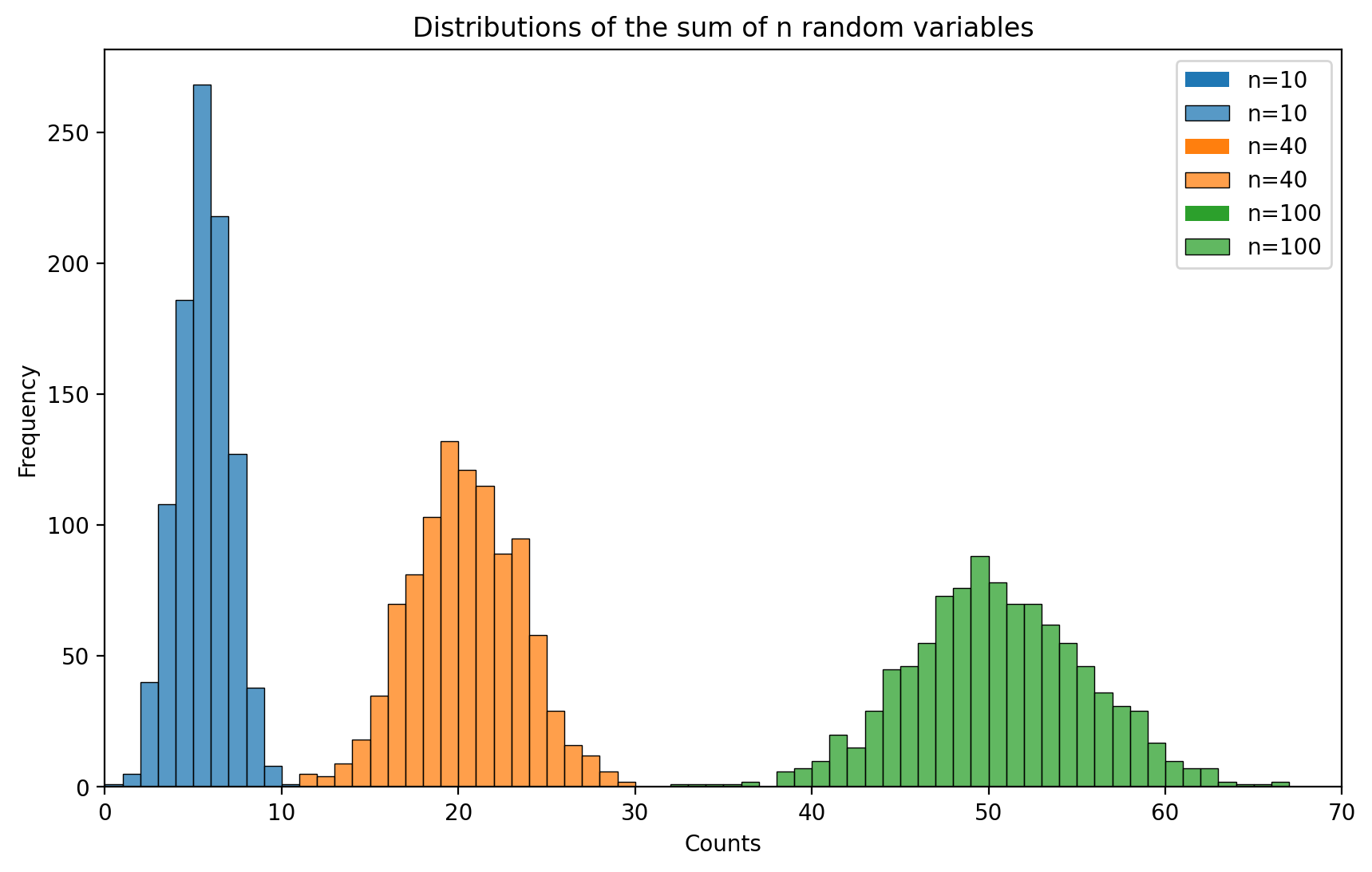
We see that for all three values of $n$ the distribution is bell-shaped.

When only 10 random variables are used to compute the sum, the distribution is centered around 5. When the sum of 40 random variables is computed, the distribution of the sum is centered around 20. With 100 random variables, it is centered around 50.

These results are in agreement with the CLT that predicts the normal distribution of the sum with mean $n\mu$, which is equal to $np=0.5n$ for these distributions.

Furthermore, the distribution with $n=10$ is the most narrow one and the one with $n=100$ has the widest spread. This in accordance with the dependence of the variance of the sum on $n$: $n{\sigma }^2$ or $np(1-p)=0.25n$ for the considered cases.

Example. Let $X_1,X_2,\dots ,X_{10}$ be independent continuous random variables, each uniformly distributed over $[0,1]$.

a. Use the CLT to approximate the distribution of $S_{10}=\sum _{i=1}^{10}{X}_i$.

b. Calculate an approximation to $P(S_{10}>6)$.

Solution.

a. To apply the CLT, we need to find $E[X_i]$ and $\text{Var}(X_i)$ first.

For a continuous uniform distribution on $[a,b]$, we know that: $$E[X_i]=\frac{a+b}{2}$$and$$\text{Var}(X_i)=\frac{(b-a{)}^2}{12}.$$

Substituting $a=0$ and $b=1$, we obtain: $E[X_i]=\frac{0+1}{2}=\frac{1}{2}$ and $\text{Var}(X_i)=\frac{(1-0{)}^2}{12}=\frac{1}{12}.$

The CLT tells us that $S_{10}=X_1+X_2+\cdots +X_{10}$ is approximately normally distrbuted with

$$E[S_{10}]=10\cdot E[X_i]=10\cdot \frac{1}{2}=5\text{ and}$$

$$\text{Var}(S_{10})=10\cdot \text{Var}(X_i)=10\cdot \frac{1}{12}=\frac{10}{12}=\frac{5}{6}.$$

b. To find $P(S_{10}>6)$, we use the normal approximation from part a.

$$P(S_{10}>6)=1-P(S_{10}\le 6)=1-P(\frac{S_{10}-5}{\sqrt{\frac{5}{6}}}\le \frac{6-5}{\sqrt{\frac{5}{6}}}).$$

Denoting the standard normal distribution by $Z$ and using the z-table we obtain $$P(S_{10}>6)=1-P(Z\le \frac{6-5}{\sqrt{\frac{5}{6}}})=1-P(Z\le \sqrt{\frac{6}{5}})=1-0.86433\approx 0.136.$$

Example. An instructor has 50 exams that will be graded in sequence. The times required to grade the 50 exams are independent, with a common distribution that has mean 20 minutes and standard deviation 4 minutes. Approximate the probability that the instructor will grade at least 25 of the exams in the first 450 minutes of work.

Solution. If we let $X_i$ be the time that it takes to grade exam $i$, then

$$S_{25}=\sum _{i=1}^{25}{X}_i$$

is the time it takes to grade the first 25 exams.

Because the instructor will grade at least 25 exams in the first 450 minutes of work if the time it takes to grade the first 25 exams is less than or equal to 450, we see that the desired probability is $P(S_{25}\le 450).$

To approximate this probability, we use the central limit theorem. Now,

$$E[S_{25}]=E\left[\sum _{i=1}^{25}{X}_i\right]=25\cdot 20=500$$

and

$$\text{Var}[S_{25}]=\text{Var}\left(\sum _{i=1}^{25}{X}_i\right)=25\cdot 16=400.$$

Consequently, with $Z$ being a standard normal random variable, we have

$$P(S_{25}\le 450)=P(\frac{S_{25}-500}{\sqrt{400}}\le \frac{450-500}{\sqrt{400}})=P(Z\le -2.5)=0.006.$$