Sampling

Today we will be discussing sampling. Resting on the probabilistics foundations of the previous lectures, this lecture marks the beginning of our study of statistics.

Population and Sample

Note

This section draws from Understanding the New Statistics, Chapter 3.

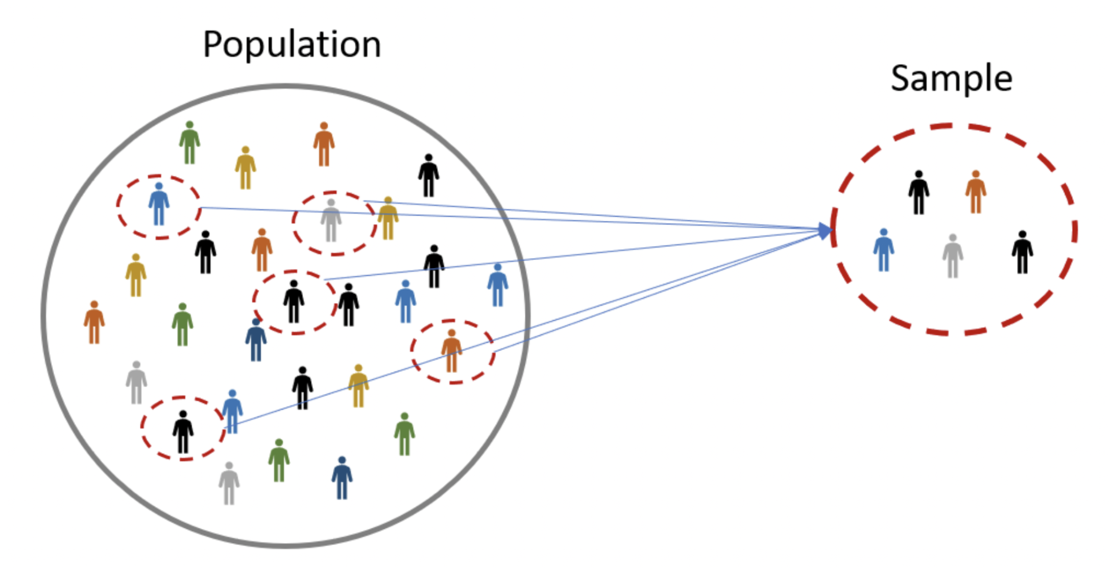
A population is the universe of possible data for a specified object. It can be people, places, objects, and many other things. It is not observable.
Example. People (or IP addresses) who have visited or will visit a website.

Typically, the size of the population is so large that if we take one object out of the population, nothing about the population changes in any perceptible way.

A sample is a subset of the population. It is observable.

Example. People who visited the website on a specific day.

We assume that we can select members of the population uniformly at random. The sample is small compared to the population, so we do not worry about the difference between sampling with replacement and sampling without replacement.

Because sampling with replacement is easier to think about in general, we will treat all samples as if they were sampled with replacement.

A statistic is anything (i.e., any function) that can be computed from the collected data sample. A statistic must be observable.

Example. The average amount of time that people spent on the website on a specific day.

The sampling distribution of a statistic is the probability distribution of that statistic when many samples are drawn.

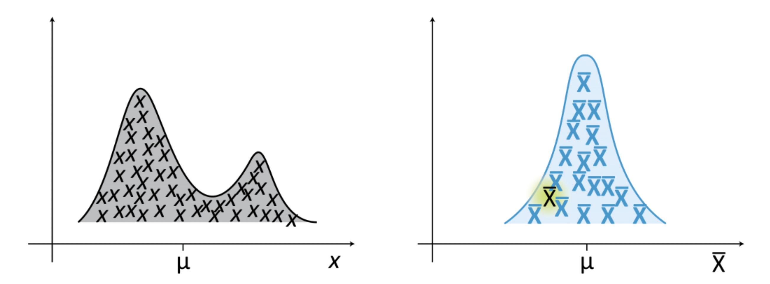
The figure shows a population distribution (left) and the corresponding sampling distribution (right) of a statistic, which in this case is the mean. The sampling distribution is obtained by drawing samples of size n from the population.

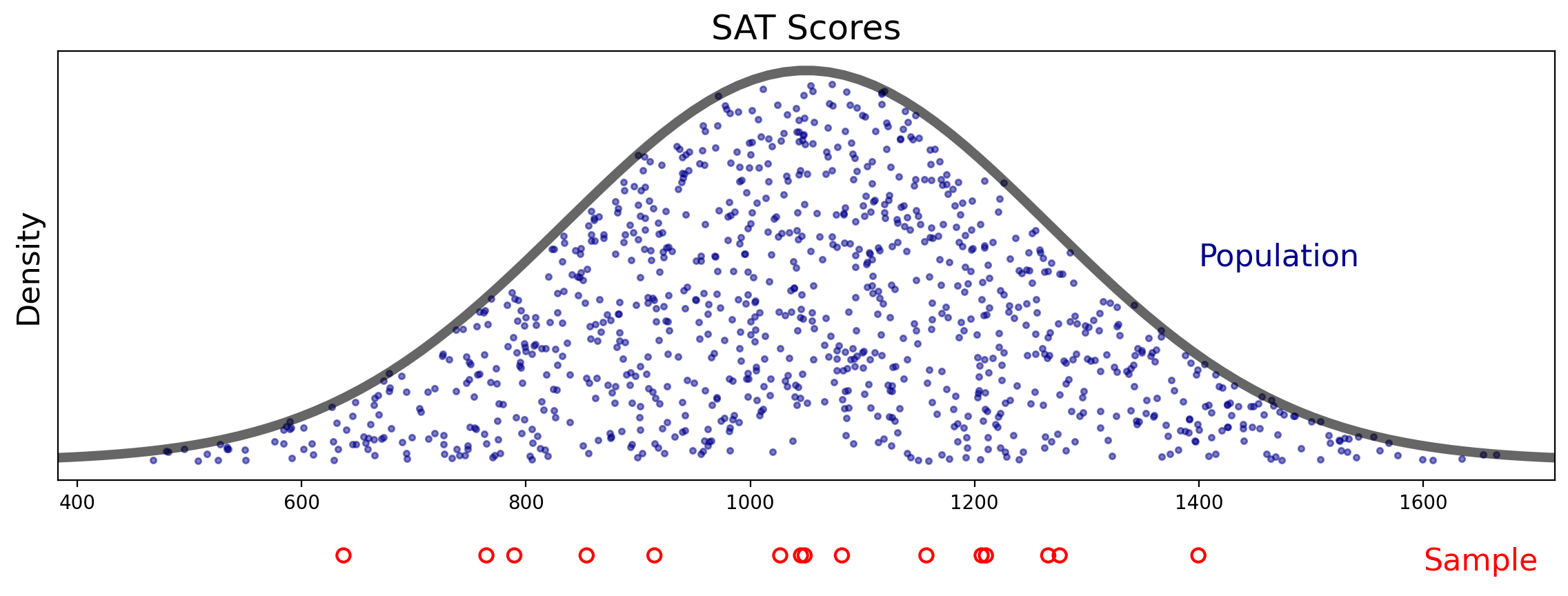
Example. Suppose you assessing success on the SAT exam. You would like to know the mean SAT score for students in your state. You choose 15 people at random from students in your state who took the exam, and you determine their scores.

In this case, the \(n = 15\) students are your sample, and the mean of their scores is a sample statistic.

Question. Should you trust your sample statistic as a reflection of the “true” population mean?

There are many things that could go wrong with your strategy:

• How do you actually choose students at random?

• How do you find students that actually took the exam?

• How do you find out the scores of the students who took the exam?

These are all valid concerns!

However, for now, we will focus our attention more narrowly on the relationship between the size of your sample and the population. So let’s assume that somehow, your sample is really random and the scores are truly reported.

Nonetheless, the mean of your sample will probably not be equal to the mean of the population.

Let’s look at the problem visually.

Note

Data on SAT Scores is available from the College Board. We’re using the mean and variance of the US national data for 2022 \((\mu = 1050, \sigma = 216)\). The College Board report shows that the data is roughly normally distributed, but for our purposes we are assuming it is exactly normally distributed.

The Distribution of the Sample Mean

Now, let’s make the assumption that the population has a normal distribution.

The population’s mean is \(\mu\) and its variance is \(\sigma^2\).

Note: both \(\mu\) and \(\sigma^2\) are unknown.

When we take \(n\) items from this distribution, then by the Central Limit Theorem, the sum of these items will be

• normally distributed

• with mean \(n\mu\)

• and variance \(n\sigma^2\).

The variances sum in this case because the items are independent – recall that was an assumption (we chose students at random).

Let’s call the sum \(S\), so

\[ S = \sum_{i=1}^n x_i \]

where \(x_i\) is one data point from the population.

Keep in mind that \(S\) is a random variable that describes a random sample.

Then \(S \sim \mathcal{N}(n\mu, n\sigma^2)\).

Now to estimate the mean of the population, we will use the mean of our sample.

Let

\[ M = \frac{1}{n} S.\]

Now, what is the distribution of \(M\)?

We are simply scaling down \(S\) by a constant. So the mean of \(M\) is

\[ \overline{M} = \frac{1}{n} \overline{S} = \frac{1}{n} \cdot n\mu = \mu. \]

What about the variane of \(M\)?

The variance is the expectation of the square of \(M - \overline{M}\).

\[ \operatorname{Var}(M) = E[(M - \overline{M})^2] = E[(S/n - \overline{S/n})^2] = \frac{1}{n^2} E[(S - \overline{S})^2] = \frac{1}{n^2} \operatorname{Var}(S)\]

So the variance goes down by a factor of \(n^2\).

\(\frac{1}{n^2} \operatorname{Var}(S) = \frac{1}{n^2}n\sigma^2 = \frac{\sigma^2}{n}\), so we find that

\[ M \sim \mathcal{N}\left(\mu, \frac{\sigma^2}{n}\right). \]

That is, the variance of the mean of the sample

• is smaller than the variance of the population,

• by a factor that depends on the number of data points in the sample.

Expressed in terms of standard deviations, the standard deviation of \(M\) is \(\sigma/\sqrt{n}\).

This is important enough that we give it a name: the standard deviation of \(M\) is called the standard error.

The stardard error is the standard deviation of the population divided by \(\sqrt{n}.\)

Let’s see how this works. Here is the mean \(M\) of our first sample:

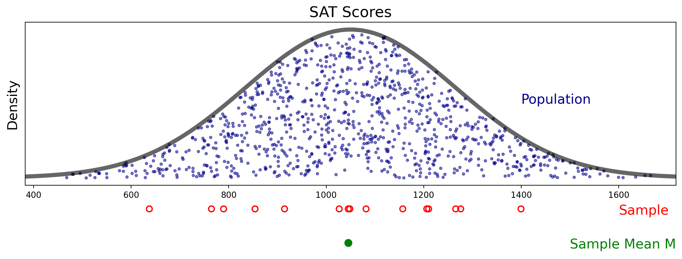
Now let’s repeat the procedure of taking \(n = 15\) samples and computing the sample mean \(M\). We’ll do this many times and show the results as a histogram.

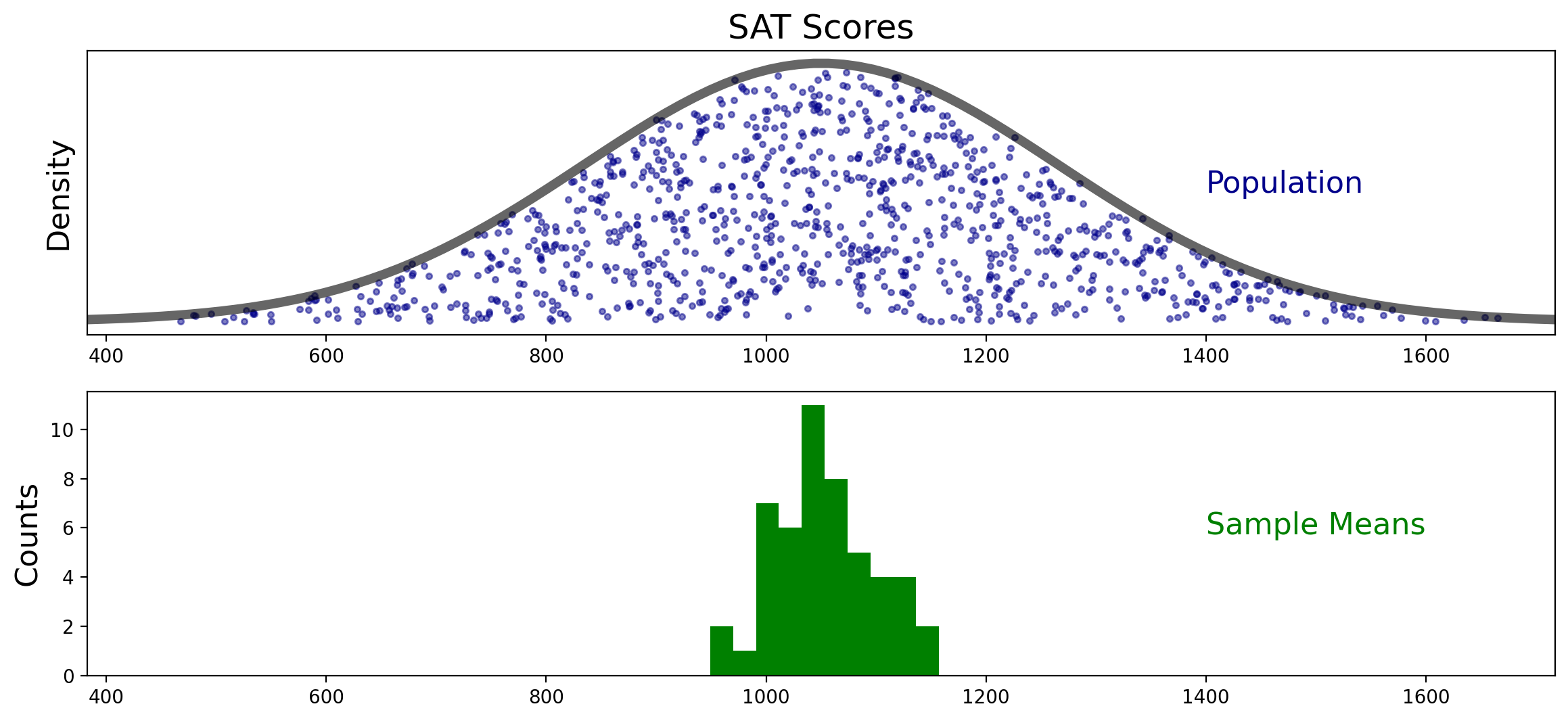
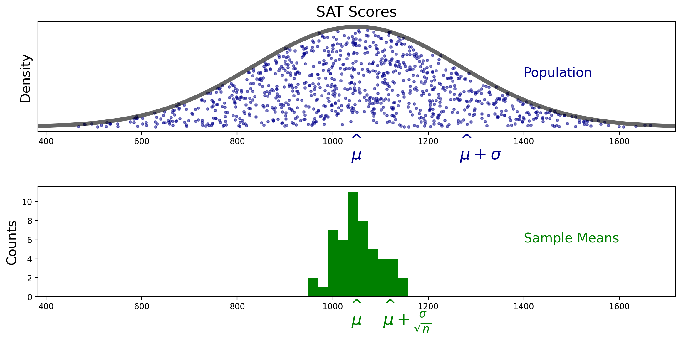
This figure shows how the sampling distribution of the mean differs from the population sample.

The sampling distribution of the mean is more concentrated around the population mean than is the population sample.

In fact, the green histogram above is showing samples from a normal distribution with mean \(\mu\) and standard deviation \(\frac{\sigma}{\sqrt{n}}\):

Effect of Sample Size

Now, the previous results showed how the sample mean \(M\) relates to the population, when \(M\) is the average of \(n = 15\) data points.

What would happen if we had taken more data points in computing \(M\)?

Intuitively, taking more data points would cause \(M\) to be a “better” estimate of the true mean \(\mu\).

We can see that in practice. Here is the histogram we get if we used 100 data points each time we compute \(M\):

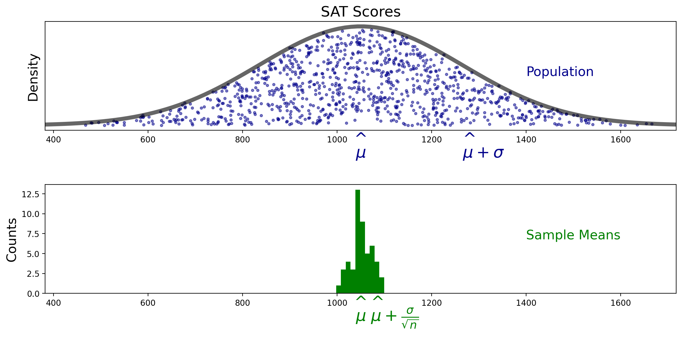
Now, the distribution of \(M\) is even more concentrated around the true mean \(\mu\).

We can be precise about this change: the standard error went from \(\frac{\sigma}{\sqrt{15}}\) to \(\frac{\sigma}{\sqrt{100}}\).