Distributions

Francis Galton's "Bean Machine"

I know of scarcely anything so apt to impress the imagination as the wonderful form of cosmic order expressed by the Law of Frequency of Error. … Whenever a large sample of chaotic elements are taken in hand and marshalled in the order of their magnitude, an unsuspected and most beautiful form of regularity proves to have been latent all along.

Francis Galton, Natural Inheritance, 1894

Useful Distributions

There are certain random variables that come up repeatedly in various situations.

We’ll study the most important ones here, and use them to illustrate some common analyses.

Each of these distributions has one or more parameters. These are settings that control the distribution.

Bernoulli Trials

(The Bernoullis were a family of accomplished mathematicians, who made a number of contributions to the study of probability.)

A Bernoulli random variable has only two outcomes: 0, and 1. It has one parameter: \(p\), which is the probability that the random variable is equal to 1.

A canonical example is flipping a weighted coin.

The coin comes up “heads” (aka “success”, aka “1”) with probability \(p\).

Note: We will often use the standard notation that the corresponding probability (“tails”, “failure”, “0”) is denoted \(q\) (i.e., \(q = 1-p\)).

Note that each coin flip is an independent event. Why do we say this?

\[\begin{split} P(\text{heads on flip }(n+1) \,\vert\, \text{heads on flip }n) = \\ P(\text{heads on flip } (n+1)) \end{split}\]

We say “the coin has no memory.”

Bernoulli Distribution

If \(X\) is a Bernoulli random variable, we say it is drawn from a Bernoulli distribution, and it can take on either the value 0 or 1.

Its distribution is therefore:

\[\begin{split} P(X) = \;\left\{\begin{array}{cr} 1-p & \text{if } X = 0\\ p & \text{if } X = 1\end{array}\right. \end{split}\]

Note that there is a particularly concise way of writing the above definition:

\[ P(X) = p^X (1-p)^{(1-X)} \]

The mean of \(X\) is \(p\) and the variance of \(X\) is \(p(1-p)\).

The Poisson Process

Now we will extend this notion to continuous time.

To start with, imagine that you flip the coin once per second.

So we expect to observe \(p\) successes per second on average.

Now, imagine that you “speed up” the coin flipping so that instead of flipping a coin once per second, you flip it \(m > 1\) times per second,

… and you simultaneously decrease the probability of success to \(p/m\).

Then you expect the same number of successes per second (i.e., \(p\)) … but events can happen at finer time intervals.

Now imagine the limit as \(m \rightarrow \infty\).

This is a mathematical abstraction in which

• an event can happen at any time instant

• an event at any time instant is equally likely

• and an event at any time instant is independent of any other time instant (it’s still a coin with no memory).

This is called a Poisson process.

In this setting, events happen at some rate \(\lambda\) that is equal to \(p\) per second.

Note that \(\lambda\) has units of inverse time, e.g., sec\(^{-1}\).

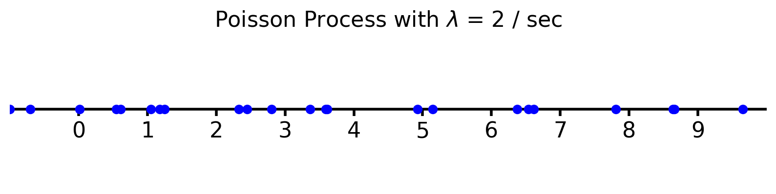
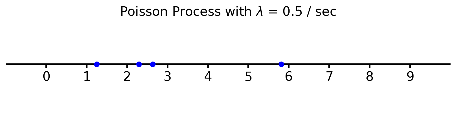
The Poisson process is a good model for things that occur randomly at some fixed rate:

• Emission of radioactive particles

• Locations of rare plants in a forest

• Arrival of phone calls in a phone network

• Errors on a communication link

• And many more

Two Kinds of Distributions

Thus we have defined two kinds of coin-flipping:

• Bernoulli trials with probability \(p\),

• Poisson process with rate \(\lambda\).

For each of these two cases (discrete and continuous time) there are two questions we can ask:

1. Given that an event has just occured, how many trials or how long until the next event?

2. In a fixed number of trials or amount of time, how many events occur?

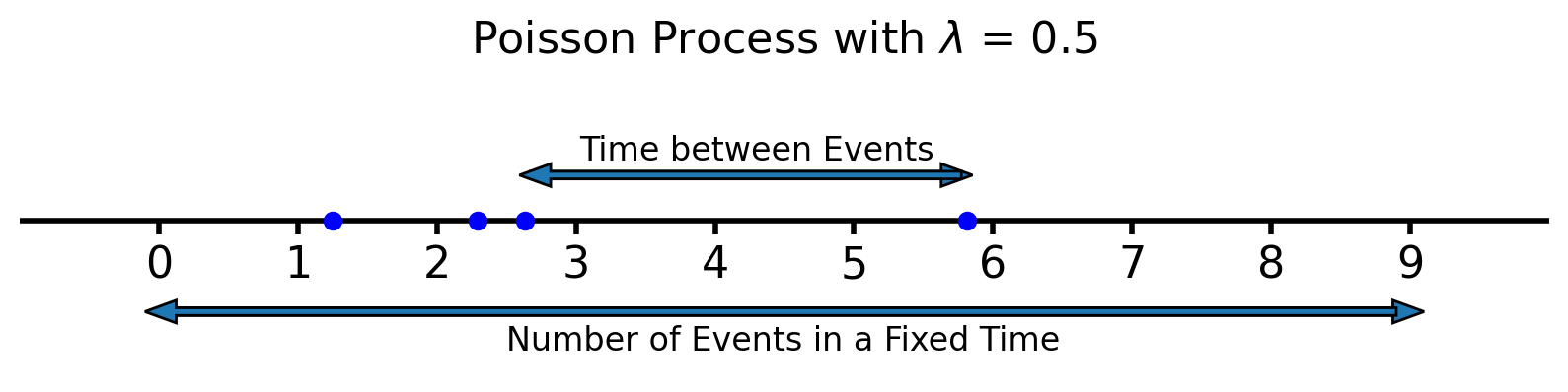
These four cases define four commonly-used random variables.

	Time (or Number of Trials) Until Event	Number of Events in Fixed Time (or Number of Trials)
Bernoulli trials	Geometric	Binomial
Poisson process	Exponential	Poisson

Each one has an associated distribution.

We’ll look at each one now.

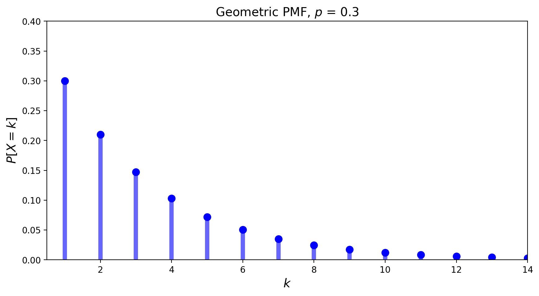
The Geometric Distribution

The geometric distribution concerns Bernoulli trials.

It answers the question: “what is the probability it takes \(k\) trials to obtain the first success?”

Its PMF is given by:

\[ P[X = k] = p(1-p)^{k-1} \qquad \text{for} \: k \geq 1.\]

Its mean is \(\mu = \frac{1}{p}\) and its variance is \(\sigma^2 = \frac{1-p}{p^2}\).

Its PMF looks like:

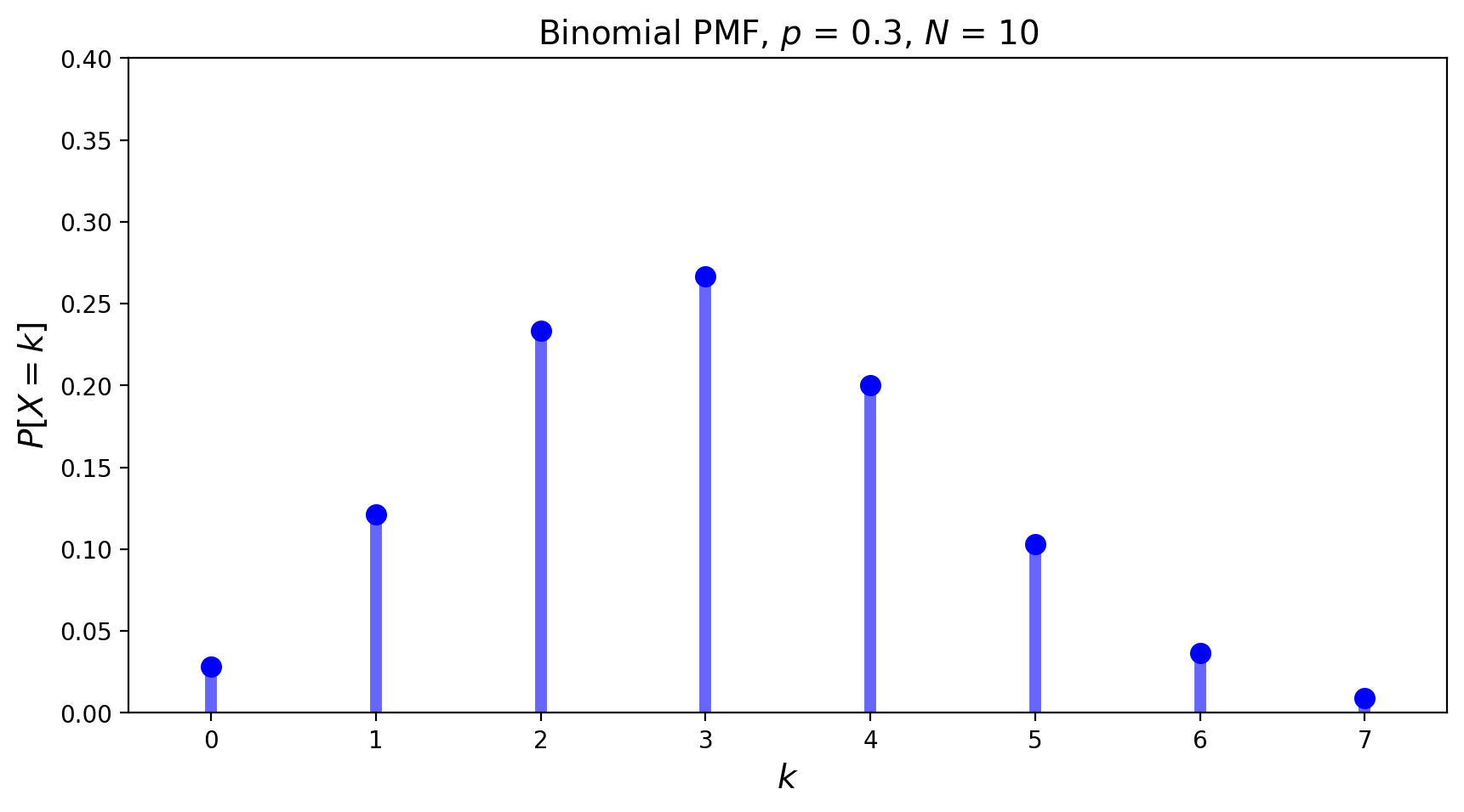
The Binomial Distribution

The Binomial also concerns Bernoulli trials.

In this experiment there are precisely \(N\) trials, and \(p\) is still the probability of a success.

Now we ask: “what is the probability there will be \(k\) successes?”

For any given sequence of \(k\) successes and \(N-k\) failures, the probability is \(p^k \;(1-p)^{N-k}\).

But there are many different such sequences: \(\binom{N}{k}\) of them in fact.

So this distribution is \(P[X=k] = \binom{N}{k}\; p^k\; (1-p)^{N-k}.\)

Its mean is \(pN\), and its variance is \(p(1-p)N\).

It’s PMF looks like:

The Exponential Distribution

Now we shift to a situation where successes occur at a fixed rate.

That is, we are considering a Poisson process.

The Exponential random variable is the analog of the geometric in the continuous case, i.e., the situation in which a success happens at some rate \(\lambda\).

This RV can be thought of as measuring the time until a success occurs.

Its PDF is:

\[ f(x) = \lambda e^{- \lambda x}.\]

The mean is \(1/\lambda\), and the variance is \(1/\lambda^2\).

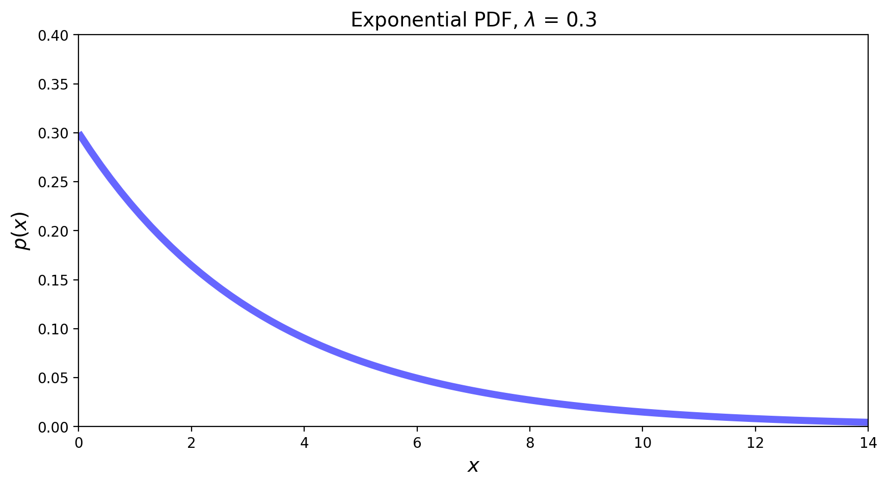
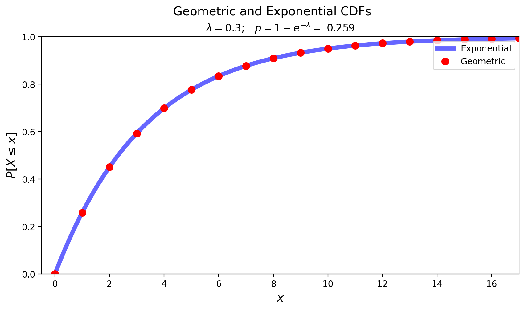
By integration we can find the CDF of the exponential:

\[ F(x) = \int_0^x \lambda e^{-\lambda s} ds = 1 - e^{-\lambda x}. \]

Notice how the Exponential is the continuous analog of the Geometric:

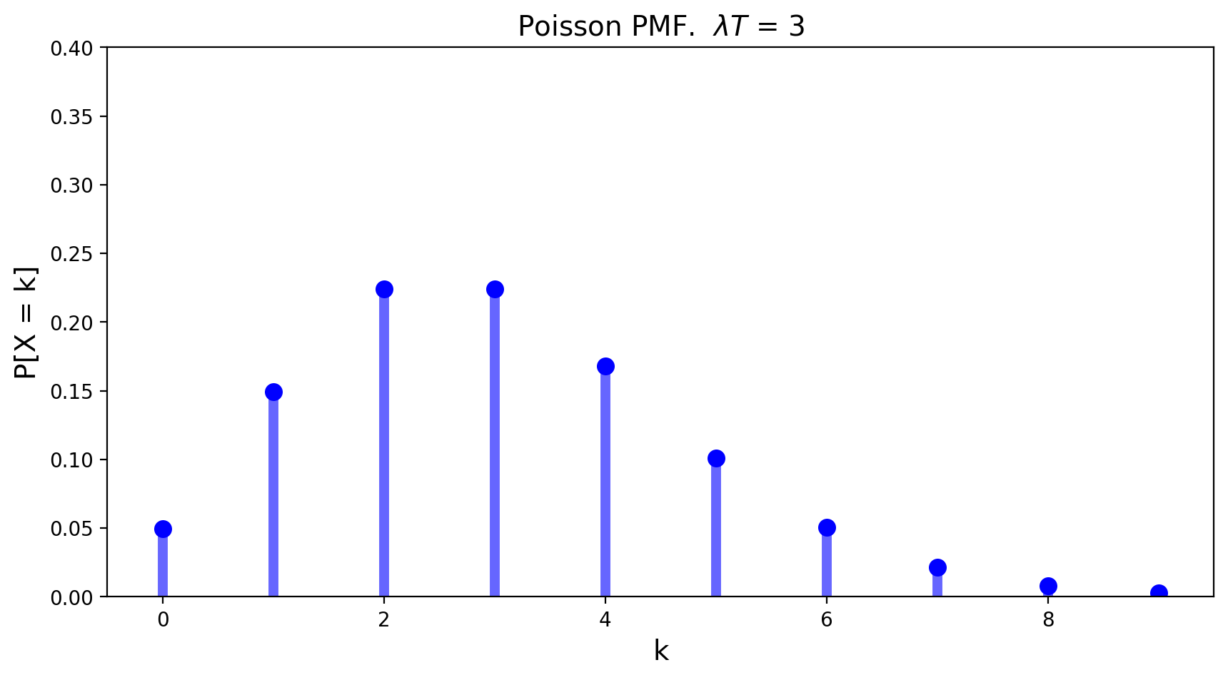
The Poisson Distribution

When we ask the question

“How many successes occur in a fixed amount of time?”,

…we get the Poisson distribution.

The Poisson distribution is the limiting form of binomial, when the number of trials goes to infinity, happening at some rate \(\lambda\).

\[ P[k \mbox{ successes in time } T] = (\lambda T)^k \frac{e^{- \lambda T}}{k!}\]

It answers the question: when events happen indepdently at some fixed rate, how many will occur in a given fixed interval?

Its mean is \(\lambda T\) and its variance is \(\lambda T\) as well.

The Poisson distribution has an interesting role in our perception of randomness (which you can read more about here).

The classic example comes from history. From the above site:

In 1898 Ladislaus Bortkiewicz, a Russian statistician of Polish descent, was trying to understand why, in some years, an unusually large number of soldiers in the Prussian army were dying due to horse-kicks. In a single army corp, there were sometimes 4 such deaths in a single year. Was this just coincidence?

To assess whether horse-kicks were random (not following any pattern) Bortkiewicz simply compared the number per year to what would be predicted by the Poisson distribution.

	Number of Deaths Per Year	Predicted Instances (Poisson)	Observed Instances
0	0.0	108.67	109.0
1	1.0	66.29	65.0
2	2.0	20.22	22.0
3	3.0	4.11	3.0
4	4.0	0.63	1.0
5	5.0	0.08	0.0
6	6.0	0.01	0.0

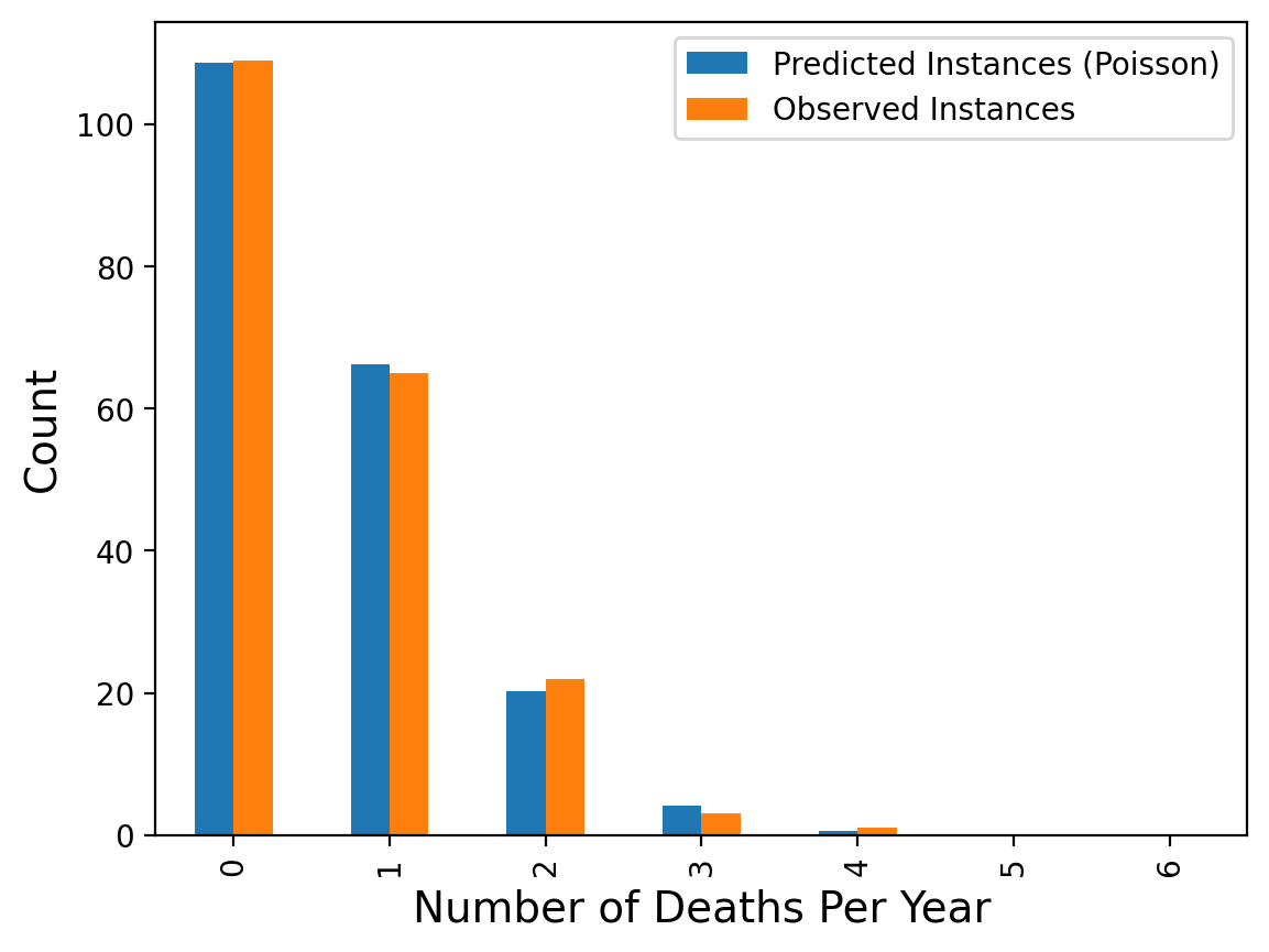
The message here is that when events occur at random, we actually tend to perceive them as clustered.

Note

This image is from Steven Pinker’s book, The Better Angels of our Nature.

Here is another example:

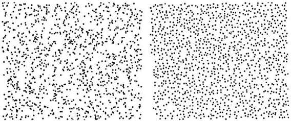
Which of these was generated by a random process ocurring equally likely everywhere?

In the left figure, the number of dots falling into regions of a given size follows the Poisson distribution.

In the right figure, the dots are too evenly dispersed to be random.

Note: From the four distributions considered so far only the exponential distribution describes a continuous random variable.

The Uniform Distribution

The uniform distribution models the case in which all outcomes are equally probable.

It can be a discrete or continuous distribution.

We have already seen the uniform distribution in the case of rolls of a fair die:

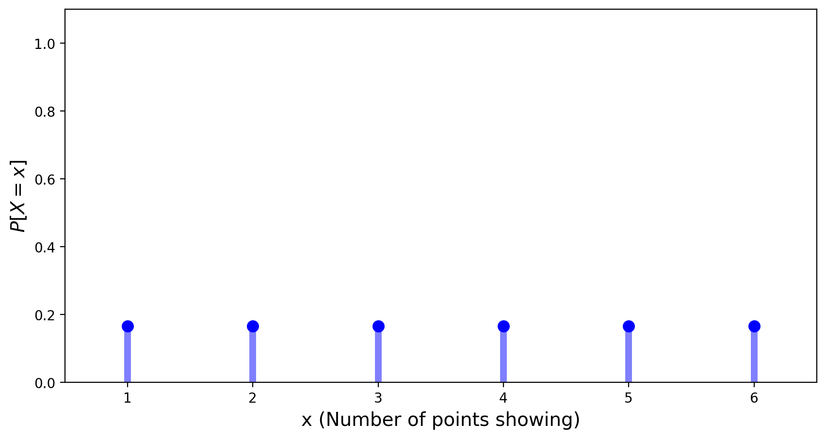
A discrete uniform distribution on interval \([a,b]\) has the PMF equal to \(\frac{1}{n}\) with \(n = b-a+1.\)

Its expected value is equal to \(\frac{a+b}{2}\) and its variance is given by \(\frac{n^2 - 1}{12}.\)

The continuous uniform distribution will be discussed in detail in the next chapter.

The Gaussian Distribution

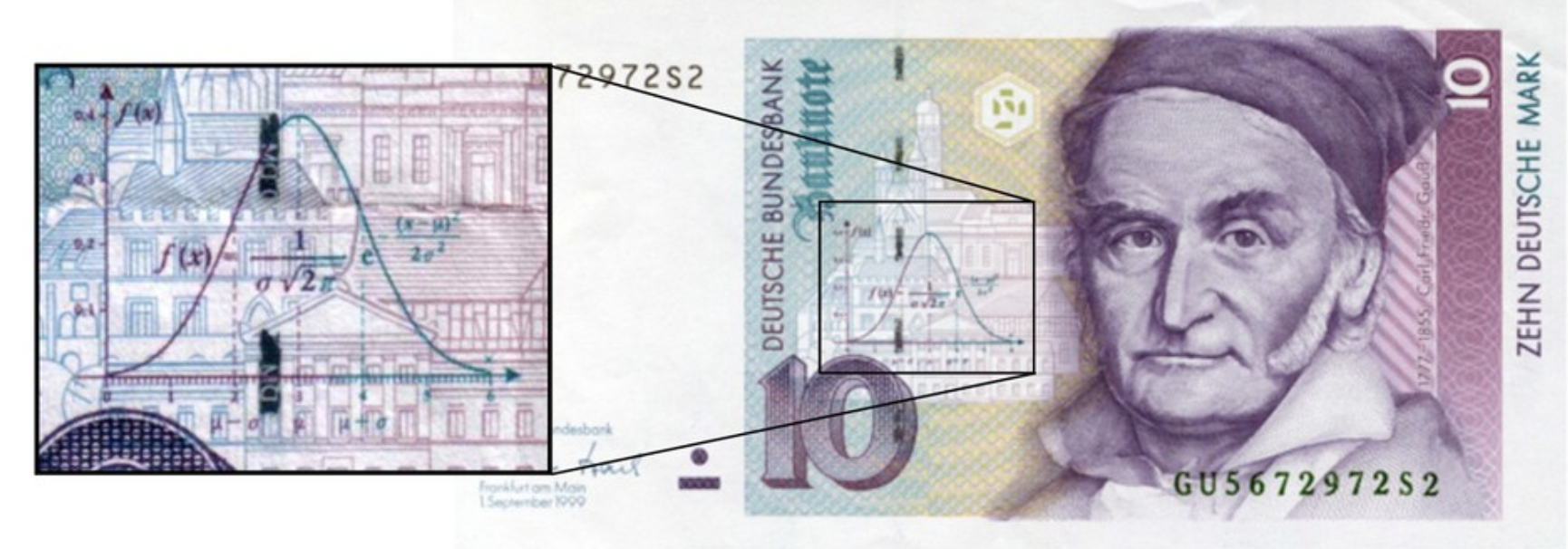
The Gaussian Distribution is also called the Normal Distribution.

We will make extensive use of Gaussian distribution!

One of reasons we will use it so much is that it is a good guess for how errors are distributed in data.

This comes from the celebrated Central Limit Theorem. Informally,

The sum of a large number of independent observations from any distribution with finite variance tends to have a Gaussian distribution.

Francis Galton's "Bean Machine"

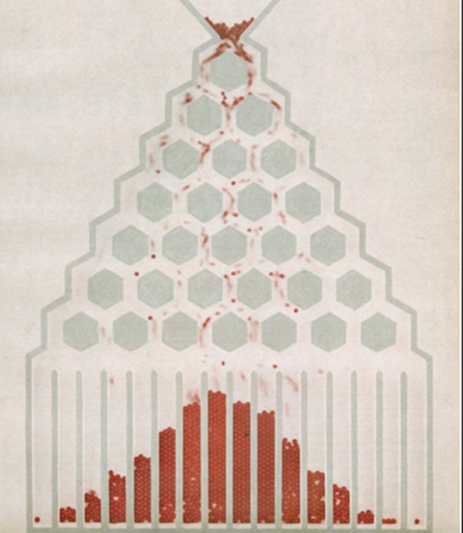
One way of thinking of the Gaussian is that it is the limit of the Binomial when \(N\) is large, that is, the limit of the sum of many Bernoulli trials.

However many other sums of random variables (not just Bernoulli trials) converge to the Gaussian as well.

The standard Gaussian distribution has mean zero and a variance (and standard deviation) of 1. The PDF of the standard Gaussian is:

\[ f(x) = \frac{1}{\sqrt{2 \pi}} e^{-x^2/2}. \]

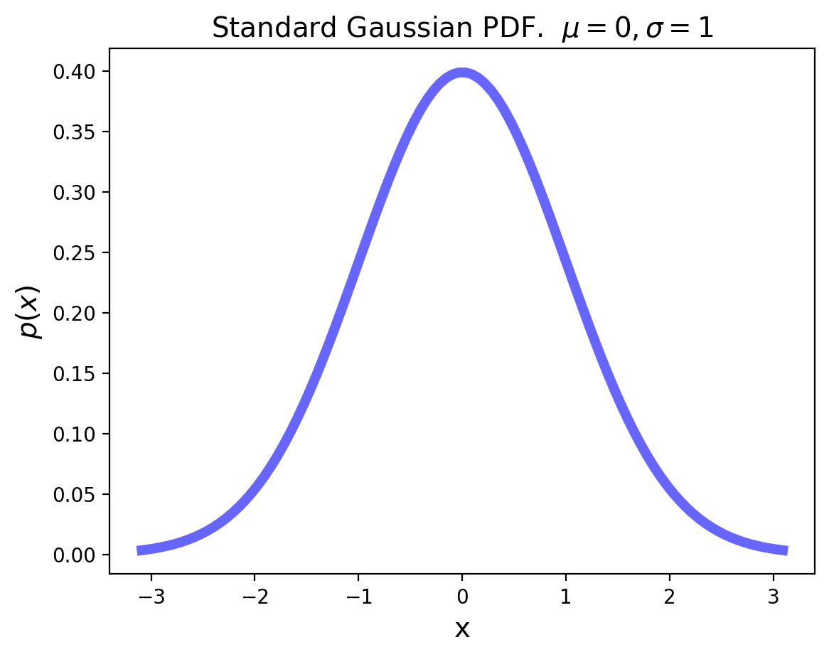
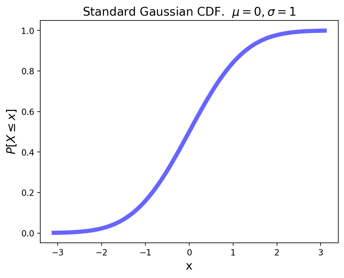
For an arbitrary Gaussian distribution with mean \(\mu\) and variance \(\sigma^2\), the PDF is simply the standard Gaussian that is relocated to have its center at \(\mu\) and its width scaled by \(\sigma\):

\[ f_{\mu,\sigma}(x) = \frac{1}{\sigma \sqrt{2 \pi}} e^{-\frac{1}{2}\left(\frac{x-\mu}{\sigma}\right)^2}. \]

As a special case, the sum of \(n\) independent Gaussian variables is Gaussian.

Thus Gaussian processes remain Gaussian after passing through linear systems.

If \(X_1\) and \(X_2\) are Gaussian, then \(X_3 = aX_1 + bX_2\) is Gaussian.

Empirical CDFs

What about when you’re working with observed data?

You can still think about the “empirical” CDF that results from your observations:

Fundementally, all it takes is sorting your numbers and counting the fraction less than each number!

values = [5, 6, 2, 1, 0, 0.5, 2, 3, 3, 4, 4, 1]
values_cdf = cdf(values)