Parameter Estimation: Estimators

Parameter Estimation: Estimators#

Some Key Concepts of Sampling#

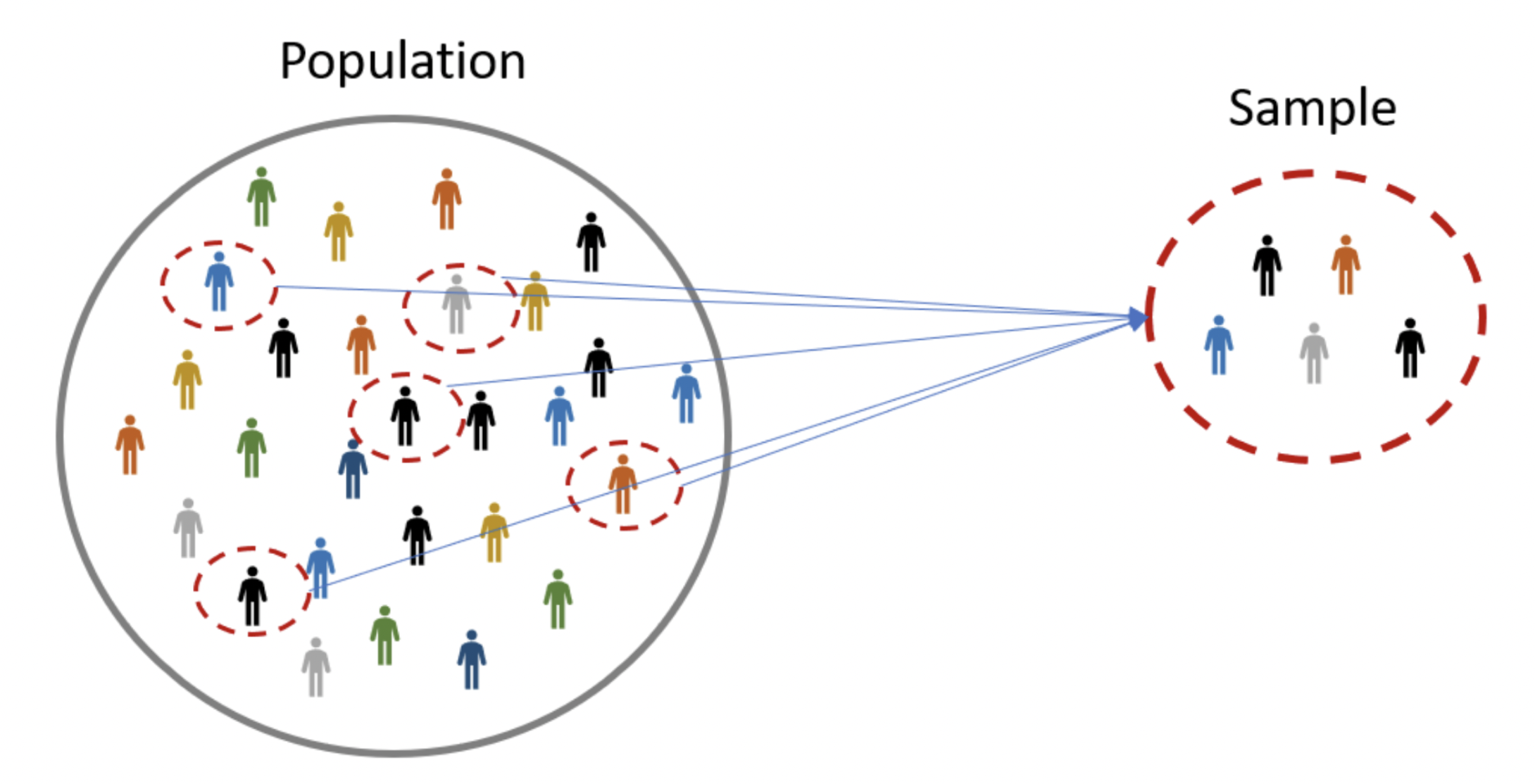
A population is the universe of possible data for a specified object. It can be people, places, objects, and many other things. It is not observable.
Example. People (or IP addresses) who have visited or will visit a website.

A sample is a subset of the population. It is observable.
Example. People who visited the website on a specific day.

What is a statistic?#

A statistic is anything (i.e., any function) that can be computed from the collected data sample. A statistic must be observable.

Parameter Estimation#

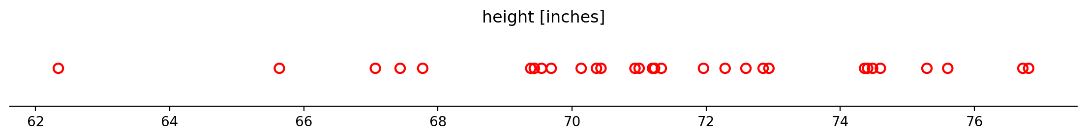
Example. We are studying the variance of height among male students at BU. Our sample of size 30 is shown below. We want to fit normal distribution $N (μ, σ^{2})$ to this data.

What values should we choose for $μ$ and $σ$ ?

_images/d338ef923d78026abdb75aa8034f21c0e016b444714bdb61adc0c8a6d7dc1f4d.png

Here, $μ$ and $σ$ are the population parameters. They are fixed but unknown.

Parameter estimation is inference about an unknown population parameter (or set of population parameters) based on a sample statistic.

Parameter estimation is a commonly used statistical technique. For instance, traffic engineers estimate the rate $λ$ of the Poisson distribution to model light traffic (individual cars move independently of each other). Their data constists of the counts of vehicles that pass a marker on a roadway during a unit of time.

In other words, we need parameter estimation when we are given some data and we want to treat it as an independent and identically distributed (or i.i.d.) sample from some population. The population has certain parameters, such as $λ$ in the above example or $μ$ and $σ$ in the example of height among male students at BU.

We will use $θ$ (which can be a scalar or a vector) to represent the parameter(s). For example, we could have $θ = (μ, σ) .$

Point Estimation#

Example. The sample average of 71.3 inches is a point estimate of the average height of male students at BU.

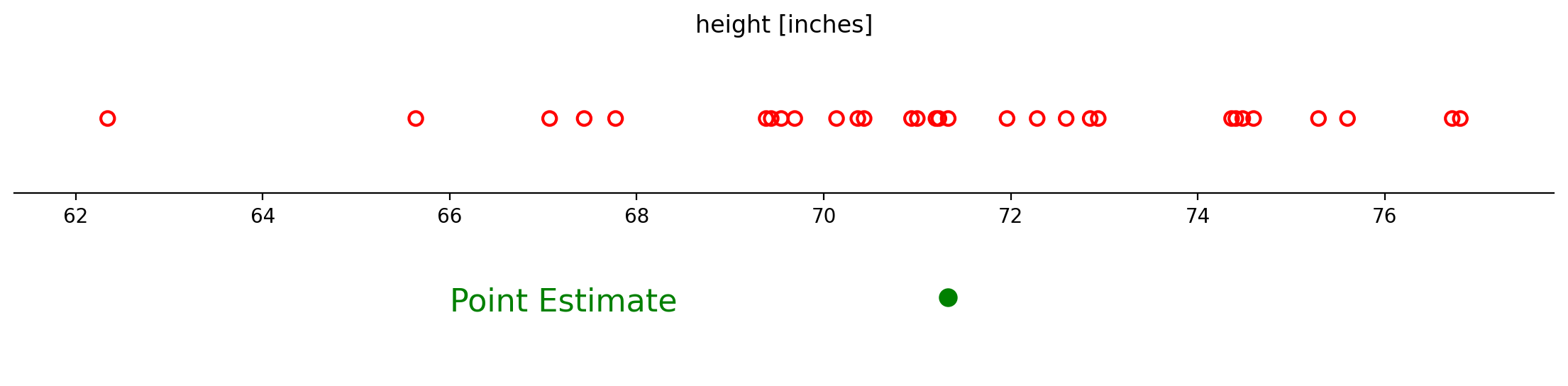
_images/77acbf730d96e5846340cd93a7456635fe3fb2e4b52edb7238cc08c1012ceaf0.png

A point estimator is a statistic that is used to estimate the unknown population parameter and whose realisation is a single point.

Let’s say our data is $x_{1}, \dots, x_{m}$ . A point estimator can be any function $g$ of the data:

{\hat{θ}}_{m} = g (x_{1}, \dots, x_{m}) .

We’ll use the hat notation ( $\hat{θ}$ ) to indicate a point estimator of $θ$ .

Note: The above definition does not require that $g$ returns a value that is close to the parameter(s) $θ$ . So any function qualifies as an estimator. However, a good estimator is a function whose output is close to $θ$ .

In the frequentist perspective on statistics, $θ$ is fixed but unknown, while $\hat{θ}$ is a function of the data. Therefore, $\hat{θ}$ is a random variable which has a probability distribution referred to as its sampling distribution.

This is a very important perspective to keep in mind; it is really the defining feature of the frequentist approach to statistics!

The sampling distribution of a statistic is the probability distribution of that statistic when we draw many samples.

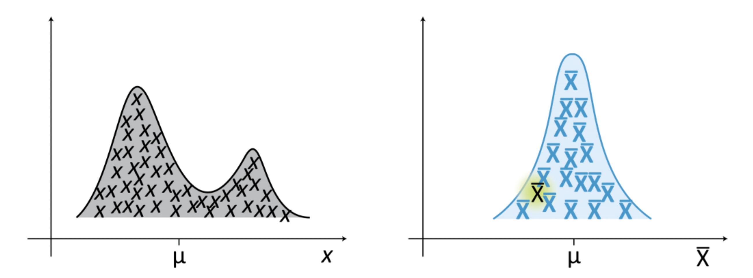
The figure shows a population distribution (left) and the corresponding sampling distribution (right) of a statistic, which in this case is the mean. The sampling distribution is obtained by drawing samples of size n from the population.

Recall that Bernoulli random variable has

only two outcomes: 0 and 1,
one parameter $p$ , which is the probability that the random variable is equal to 1,
mean equal to $p$ and variance equal to $p (1 - p)$ ,
PMF: $p^{x} (1 - p)^{(1 - x)} .$

Example. Consider data sample $x_{1}, \dots, x_{m}$ drawn independently and identically from a Bernoulli distribution with mean $θ$ :

p (x_{i}; θ) = θ^{x_{i}} {(1 - θ)}^{(1 - x_{i})} .

A common estimator for $θ$ is the mean of the realizations:

{\hat{θ}}_{m} = g (x_{1}, \dots, x_{m}) = \frac{1}{m} \sum_{i = 1}^{m} x_{i} .

Bias and Variance#

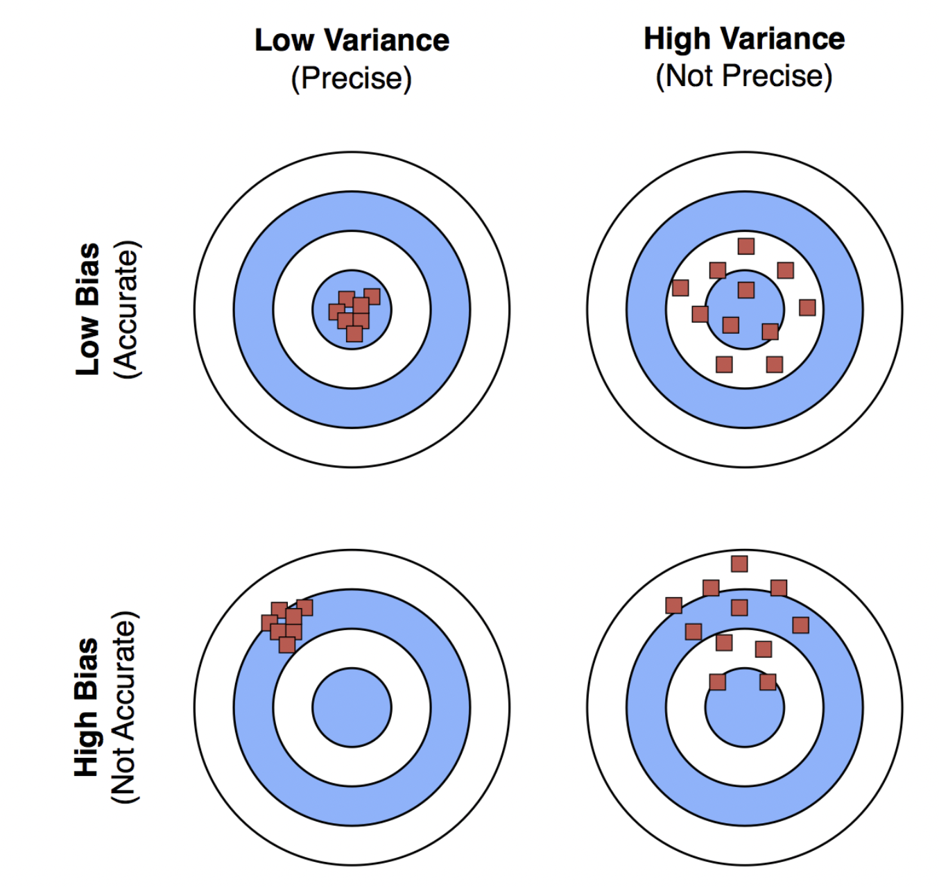
We use two criteria to describe an estimator: bias and variance.

Bias measures the difference between the expected value of the estimator and the true value of the parameter, while variance measures how much the estimator can vary as a function of the data sample.

Bias. The bias of an estimator is defined as:

bias (\hat{θ}) = E [\hat{θ}] - θ,

where the expectation is over the data (seen as realizations of a random variable) and $θ$ is the true underlying value of $θ$ used to define the data-generating distribution.

An estimator is said to be unbiased if $bias (\hat{θ}) = 0$ , or in other words $E [\hat{θ}] = θ$ .

Continuing our example for the mean of the Bernoulli:

\begin{array}{r} bias ({\hat{θ}}_{m}) = E [{\hat{θ}}_{m}] - θ \\ = E [\frac{1}{m} \sum_{i = 1}^{m} x_{i}] - θ \end{array}

\begin{array}{r} = \frac{1}{m} \sum_{i = 1}^{m} E [x_{i}] - θ \\ = \frac{1}{m} \sum_{i = 1}^{m} (θ) - θ \end{array}

\begin{array}{r} = \frac{1}{m} (m θ) - θ \\ = θ - θ = 0. \end{array}

So we have proven that this estimator of $θ$ is unbiased.

Variance. The variance of an estimator is simply the variance

Var (\hat{θ}) = Var (g (x_{1}, \dots, x_{m}))

where $g (x_{1}, \dots, x_{m})$ is a function of the data set.

Remember that the data set is random; it is assumed to be an i.i.d. sample of some distribution.

Recall:
I. If $Var (X)$ exists and $Y = a X + b$ , then $Var (Y) = a^{2} Var (X)$ .
II. If $X_{1}, X_{2}, \dots, X_{m}$ are i.i.d., then $Var (\sum_{i = 1}^{m} X_{i}) = m Var (X_{1}) .$

Let us return again to our example where the sample is drawn from the Bernoulli distribution and the estimator ${\hat{θ}}_{m} = \frac{1}{m} \sum_{i = 1}^{m} x_{i}$ is simply the mean of $m$ observations.

So we see that the variance of the mean is:

Var ({\hat{θ}}_{m}) = Var (\frac{1}{m} \sum_{i = 1}^{m} x_{i}) = \frac{1}{m^{2}} Var (\sum_{i = 1}^{m} x_{i})

= \frac{1}{m^{2}} m Var (x_{i}) = \frac{1}{m} θ (1 - θ) .

This has a desirable property: as the number of data points $m$ increases, the variance of the estimate decreases.

Note: It can be shown that for a sample $x_{1}, \dots, x_{m}$ drawn independently and identically from any population with mean $μ$ and variance $σ^{2}$ . The sample mean, $\frac{1}{m} \sum_{i = 1}^{m} x_{i}$ , is an unbiased estimator of the population mean and has variance $\frac{σ^{2}}{m}$ .

What if we use ${\hat{β}}_{m} = c$ , where $c$ is a constant, to estimate the population mean in our Bernoulli example?

The variance of this estimator is equal to

Var ({\hat{β}}_{m}) = Var (c) = 0.

However, the bias in this case is equal to

bias ({\hat{β}}_{m}) = E [{\hat{β}}_{m}] - θ = E [c] - θ = c - θ .

The estimator ${\hat{β}}_{m} = c$ is biased.

Mean Squared Error#

Consider two estimators, $g$ and $h$ , each of which are used as estimates of a certain parameter $θ$ .

Let us say that these estimators show the following distributions:

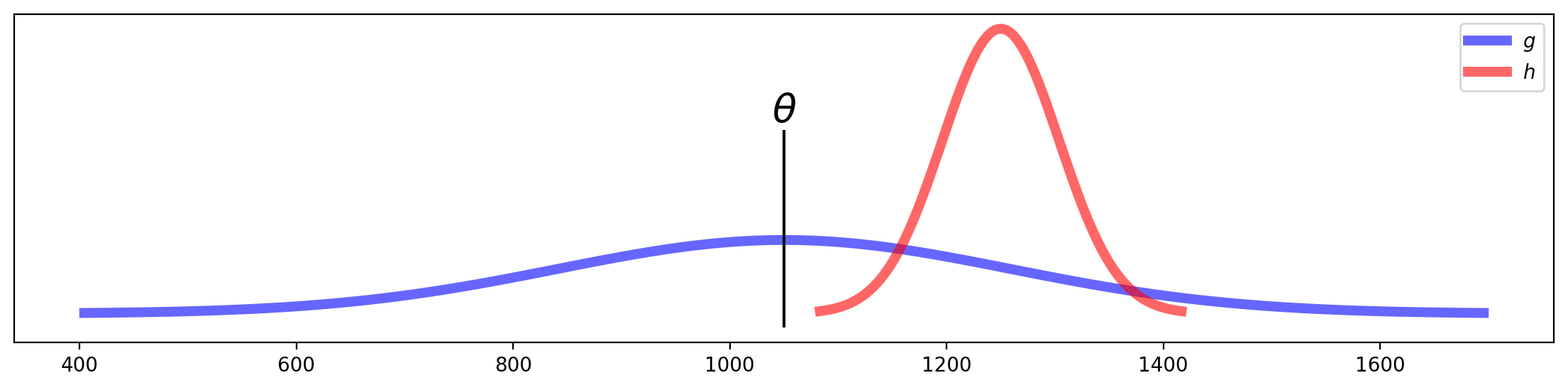
_images/653e9ccbf95abd7f9fdbc3ef2ad8d52ada728f600a530edc0d67441f2077a341.png

The figure shows that estimator $h$ has low variance, but is biased. Meanwhile, estimator $g$ is unbiased, but has high variance.

Which is better?

The answer of course depends, but there is a single criterion we can use to try to balance these two kinds of errors.

It is Mean Squared Error.

MSE (\hat{θ}) = E [{(\hat{θ} - θ)}^{2}] .

This measures the “average distance squared” between the estimator and the true value.

It is a good single number for evaluating an estimator, because it turns out that:

MSE (\hat{θ}) = bias {(\hat{θ})}^{2} + Var (\hat{θ}) .

For example, the two estimators $g$ and $h$ in the plot above have approximately the same MSE.

We have already shown that for sample $x_{1}, \dots, x_{m}$ that is drawn independently and identically from a Bernoulli distribution with mean $θ$ , the estimator ${\hat{θ}}_{m} = \frac{1}{m} \sum_{i = 1}^{m} x_{i}$ is unbiased and and has variance $\frac{1}{m} θ (1 - θ)$ . Therefore,

M S E ({\hat{θ}}_{m}) = Var ({\hat{θ}}_{m}) = \frac{1}{m} θ (1 - θ) .

Python example#

Consider the following i.i.d. data sample of size 35.

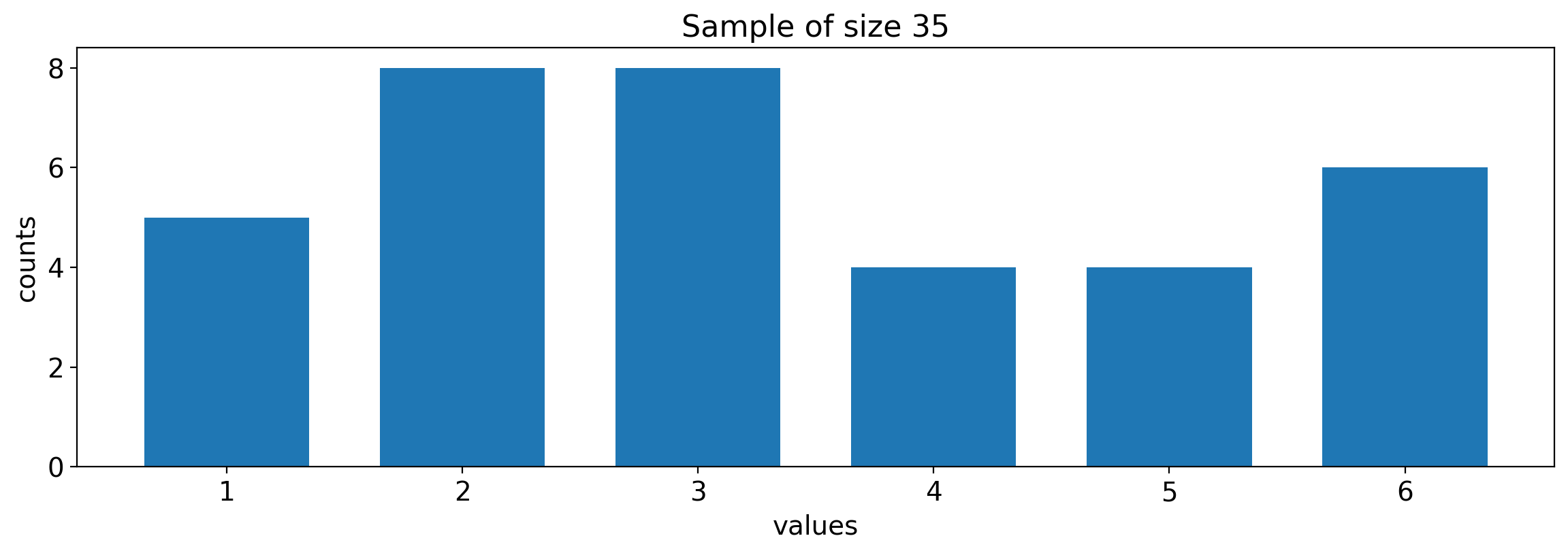
_images/46ca1abdc3e816197cbbe45ec4a447d8f79ed7e5f8506187c8fc37f16cf97e4c.png

Is the sample from a discrete uniform distribution? Do the values range from 1 to 6?

Discrete uniform distribution:

$n = b - a + 1$

parameters: $a$ and $b$
mean: $\frac{a + b}{2}$
variance: $\frac{n^{2} - 1}{12} = \frac{(b - a + 1)^{2} - 1}{12}$

If the population distribution is $U (1, 6)$ , the population mean should be equal to 3.5 and the population variance should be approximately 2.917.

We can use the provided sample to estimate the population mean and variance.

Note: We are not fitting $U (1, 6)$ to the sample. We are simply looking for point estimates for the population mean and variance.

We discussed earlier that regardless of the population distribution, the sample mean is an unbiased estimator of the population mean and its variance is inversely proportional to the size of the sample.

Thus we will use the sample average to estimate the population mean:

\hat{θ} = \frac{1}{35} \sum_{i = 1}^{35} x_{i} .

# compute the sample mean
mu_hat = np.mean(s)
print(f'The estimate of the population mean is equal to {mu_hat:.4}.')

The estimate of the population mean is equal to 3.343.

What about the population variance? Can it be estimated by

\frac{\sum_{i = 1}^{m} {(x_{i} - \overset{―}{x})}^{2}}{m} = \frac{\sum_{i = 1}^{35} {(x_{i} - \overset{―}{x})}^{2}}{35} ?

# compute the variance of the sample (without Bessel's correction)
sig2_hat_1 = np.var(s, axis = 0, ddof = 0)
print(f'The biased sample variance is equal to {sig2_hat_1:0.4}.')

The biased sample variance is equal to 2.797.

We will see later in this lecture that this estimator systematically underestimates the population variance. Bessel’s correction is required to obtain an unbiased estimator:

\frac{\sum_{i = 1}^{m - 1} {(x_{i} - \overset{―}{x})}^{2}}{m - 1} = \frac{\sum_{i = 1}^{34} {(x_{i} - \overset{―}{x})}^{2}}{34} .

The above expression is known as sample variance.

# compute the sample variance (with Bessel's correction)
sig2_hat_2 = np.var(s, axis = 0, ddof = 1)
print(f'The unbiased sample variance is equal to {sig2_hat_2:0.4}.')

The unbiased sample variance is equal to 2.879.

Conclusion. Based on the provided sample, the population mean can be estimated by 3.343 and the population variance can be estimated by 2.879. These values are close to 3.5 and 2.917, respectively. Therefore, $U (1, 6)$ can be considered a “good guess” for the population distribution.

Effect of Bessel’s correction#

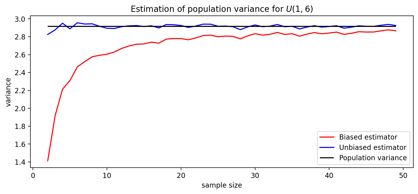
_images/322b27b51b0f839a2817df544b1ddaab822831f674e313c02766d7b6d374a70e.png

Note: The $y$ -axis corresponds to the variance that is obtained by taking an average over 1000 samples for each sample size.