Applications of the SVD

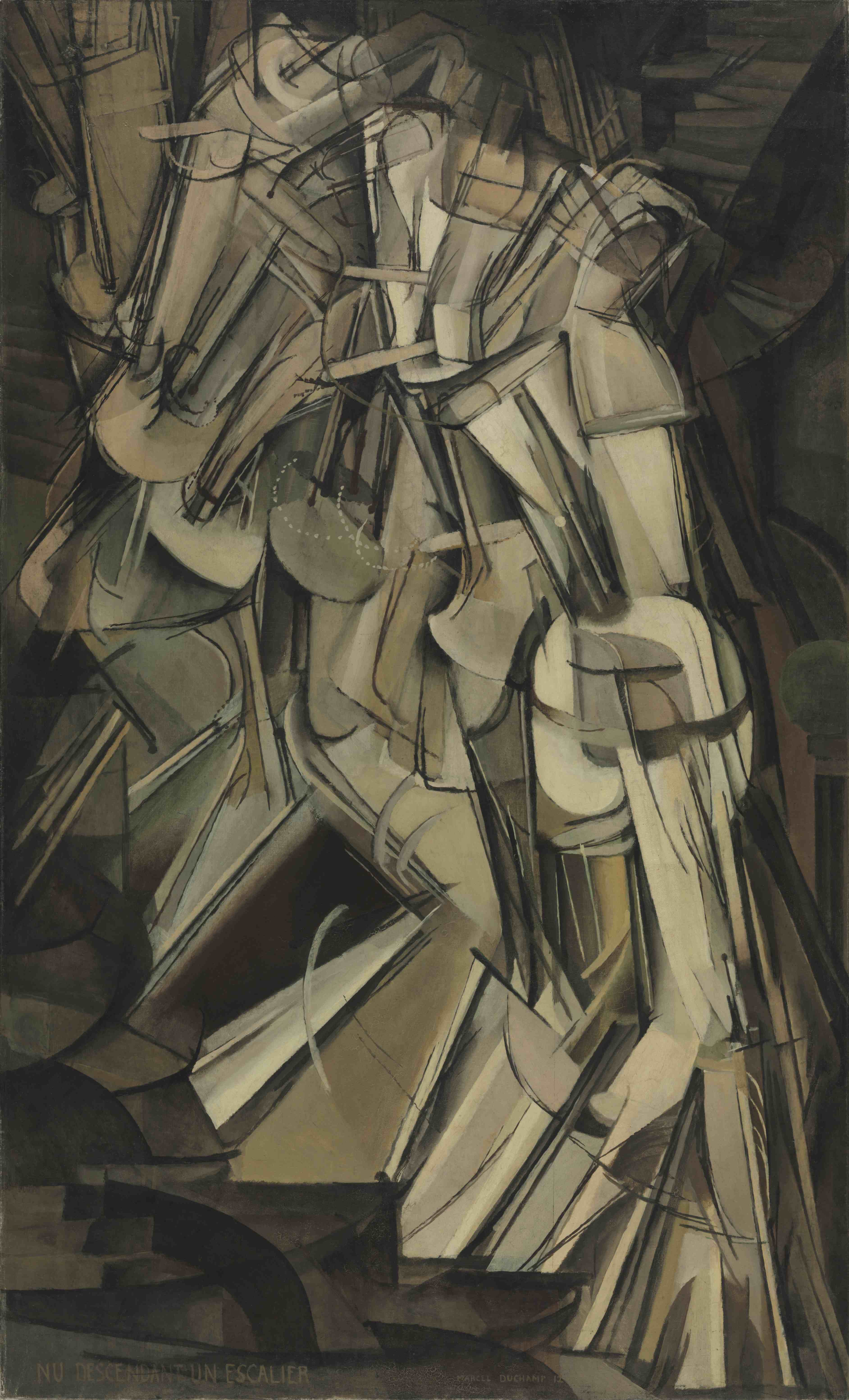
In “Nude Descending a Staircase” Marcel Duchamp captures a four-dimensional object on a two-dimensional canvas. Accomplishing this without losing essential information is called dimensionality reduction.

Nude Descending a Staircase by Marcel Duchamp (1887-1968) - Philadelphia Museum of Art, PD-US

Image from Wikipedia

The Singular Value Decomposition is the “Swiss Army Knife” and the “Rolls Royce” of matrix decompositions.

– Diane O’Leary

Today we will concern ourselves with the “Swiss Army Knife” aspect of the SVD.

Our focus today will be on applications to data analysis.

So today we will be thinking of matrices as data.

(Rather than thinking of matrices as linear operators.)

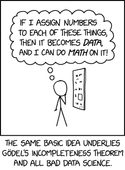
Image Credit: xkcd

As a specific example, here is a typical data matrix. This matrix could be the result of measuring a collection of data objects, and noting a set of features for each object.

\[{\text{$m$ data objects}}\left\{\begin{array}{c}\;\\\;\\\;\\\;\\\;\end{array}\right.\;\;\overbrace{\left[\begin{array}{ccccc} \begin{array}{c}a_{11}\\\vdots\\a_{i1}\\\vdots\\a_{m1}\end{array}& \begin{array}{c}\dots\\\ddots\\\dots\\\ddots\\\dots\end{array}& \begin{array}{c}a_{1j}\\\vdots\\a_{ij}\\\vdots\\a_{mj}\end{array}& \begin{array}{c}\dots\\\ddots\\\dots\\\ddots\\\dots\end{array}& \begin{array}{c}a_{1n}\\\vdots\\a_{in}\\\vdots\\a_{mn}\end{array} \end{array}\right]}^{n \text{~features}}\]

For example, rows could be people, and columns could be movie ratings.

Or rows could be documents, and columns could be words within the documents.

Recap of SVD

To start discussing the set of tools that SVD provides for analyzing data, let’s remind ourselves what the SVD is.

Today we’ll work exclusively with the reduced SVD.

Here it is again, for the case where \(A\) is \(m \times n\), and \(A\) has rank \(r\).

In that case, the reduced SVD looks like this, with singular values on the diagonal of \(\Sigma\):

\(\tiny {\small m}\left\{\begin{array}{c}\;\\\;\\\;\\\;\\\;\end{array}\right.\;\;\overbrace{\left[\begin{array}{cccc}\begin{array}{c}\vdots\\\vdots\\{\bf a_1}\\\vdots\\\vdots\end{array}&\begin{array}{c}\vdots\\\vdots\\{\bf a_2}\\\vdots\\\vdots\end{array}&\dots&\begin{array}{c}\vdots\\\vdots\\{\bf a_n}\\\vdots\\\vdots\end{array}\\\end{array}\right]}^{\small n} = \overbrace{\left[\begin{array}{ccc}\vdots&&\vdots\\\vdots&&\vdots\\\mathbf{u}_1&\cdots&\mathbf{u}_r\\\vdots&&\vdots\\\vdots&&\vdots\end{array}\right]}^{\small r} \times \overbrace{\left[\begin{array}{ccc}\sigma_1& &\\&\ddots&\\&&\sigma_r\end{array}\right]}^{\small r} \times \overbrace{\left[\begin{array}{ccccc}\dots&\dots&\mathbf{v}_1&\dots&\dots\\&&\vdots&&\\\dots&\dots&\mathbf{v}_r&\dots&\dots\end{array}\right]}^{\small n}\)

\[\Large\overset{m\,\times\, n}{A^{\vphantom{T}}} = \overset{m\,\times\, r}{U^{\vphantom{T}}}\;\;\overset{r\,\times\, r}{\Sigma^{\vphantom{T}}}\;\;\overset{r\,\times\, n}{V^T}\]

Approximating a Matrix

To understand the power of SVD for analyzing data, it helps to think of it as a tool for approximating one matrix by another, simpler, matrix.

To talk about when one matrix approximates another, we need a “length” for matrices.

We will use the Frobenius norm.

The Frobenius norm is just the usual vector norm, treating the matrix as if it were a vector.

In other words, the definition of the Frobenius norm of \(A\), denoted \(\Vert A\Vert_F\), is:

\[\Vert A\Vert_F = \sqrt{\sum a_{ij}^2}.\]

The approximations we’ll discuss are low-rank approximations.

Recall that the rank of a matrix \(A\) is the largest number of linearly independent columns of \(A\).

Or, equivalently, the dimension of \(\operatorname{Col} A\).

Let’s define the rank-\(k\) approximation to \(A\):

When \(k < \operatorname{Rank}A\), the rank-\(k\) approximation to \(A\) is the closest rank-\(k\) matrix to \(A\), i.e.,

\[A^{(k)} =\arg \min_{\operatorname{Rank}B = k} \Vert A-B\Vert_F.\]

Why is a rank-\(k\) approximation valuable?

The reason is that a rank-\(k\) matrix may take up much less space than the original \(A\).

\(\small {\normalsize m}\left\{\begin{array}{c}\;\\\;\\\;\\\;\\\;\end{array}\right.\;\;\overbrace{\left[\begin{array}{cccc}\begin{array}{c}\vdots\\\vdots\\{\bf a_1}\\\vdots\\\vdots\end{array}&\begin{array}{c}\vdots\\\vdots\\{\bf a_2}\\\vdots\\\vdots\end{array}&\dots&\begin{array}{c}\vdots\\\vdots\\{\bf a_n}\\\vdots\\\vdots\end{array}\\\end{array}\right]}^{\normalsize n} = \overbrace{\left[\begin{array}{cc}\vdots&\vdots\\\vdots&\vdots\\\sigma_1\mathbf{u}_1&\sigma_k\mathbf{u}_k\\\vdots&\vdots\\\vdots&\vdots\end{array}\right]}^{\normalsize k} \times \overbrace{\left[\begin{array}{ccc}\dots&\mathbf{v}_1&\dots\\\dots&\mathbf{v}_k&\dots\end{array}\right]}^{\normalsize n}\)

Notice that:

• \(A\) takes space \(mn\)
• but the rank-\(k\) approximation only takes space \((m+n)k\).

For example, if A is \(1000 \times 1000\), and \(k=10\), then

• A takes space \(1000000\)
• while the rank-\(k\) approximation takes space \(20000\),

So the rank-\(k\) approximation is just 2% the size of \(A\).

The fact that the SVD finds the best rank-\(k\) approximation to any matrix is called the Eckart-Young-Mirsky Theorem. You can find a proof of the theorem here. In fact it is true for the Frobenius norm (the norm we are using here) as well as another matrix norm, the spectral norm.

More good resources on how to understand SVD as a data approximation method are here and here.

The key to using the SVD for matrix approximation is as follows:

The best rank-k approximation to any matrix can be found via the SVD.

In fact, for an \(m\times n\) matrix \(A\), the SVD does two things:

  1. It gives the best rank-\(k\) approximation to \(A\) for every \(k\) up to the rank of \(A\).

  2. It gives the distance of the best rank-\(k\) approximation \(A^{(k)}\) from \(A\) for each \(k\).

When we say “best”, we mean in terms of Frobenius norm \(\Vert A-A^{(k)}\Vert_F\),

and by distance we mean the same quantity, \(\Vert A-A^{(k)}\Vert_F\).

How do we use SVD to find the best rank-\(k\) approximation to \(A\)?

Conceptually, we “throw away” the portions of the SVD having the smallest singular values.

More specifically: in terms of the singular value decomposition,

\[ A = U\Sigma V^T, \]

the best rank-\(k\) approximation to \(A\) is formed by taking

• \(U' =\) the \(k\) leftmost columns of \(U\),
• \(\Sigma ' =\) the \(k\times k\) upper left submatrix of \(\Sigma\), and
• \((V')^T=\) the \(k\) upper rows of \(V^T\),

and constructing

\[A^{(k)} = U'\Sigma'(V')^T.\]

The distance (in Frobenius norm) of the best rank-\(k\) approximation \(A^{(k)}\) from \(A\) is equal to

\[\sqrt{\sum_{i=k+1}^r\sigma^2_i}.\]

Notice that this quantity is summing over the singular values beyond \(k\).

What this means is that if, beyond some \(k\), all of the singular values are small, then \(A\) can be closely approximated by a rank-\(k\) matrix.

Signal Compression

When working with measurement data, ie measurements of real-world objects, we find that data is often approximately low-rank.

In other words, a matrix of measurements can often be well approximated by a low-rank matrix.

Classic examples include

• measurements of human abilities - eg, psychology
• measurements of human preferences – eg, movie ratings, social networks
• images, movies, sound recordings
• genomics, biological data
• medical records
• text documents

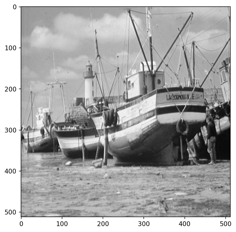
For example, here is a photo.

We can think of this as a \(512\times 512\) matrix \(A\) whose entries are grayscale values (numbers between 0 and 1).

Let’s look at the singular values of this matrix.

We compute \(A = U\Sigma V^T\) and look at the values on the diagonal of \(\Sigma\).

This is often called the matrix’s “spectrum.”

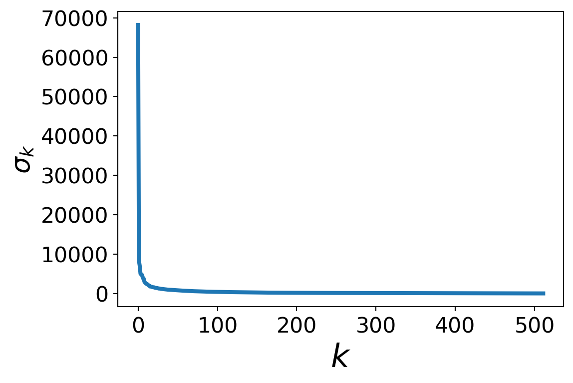
What is this telling us?

Most of the singular values of \(A\) are quite small.

Only the first few singular values are large – up to, say, \(k\) = 40.

Remember that the error we get when we use a rank-\(k\) approximation is

\[\Vert A-A^{(k)}\Vert_F = \sqrt{\sum_{i=k+1}^r\sigma^2_i}.\]

So we can use the singular values of \(A\) to compute the relative error over a range of possible approximations \(A^{(k)}\).

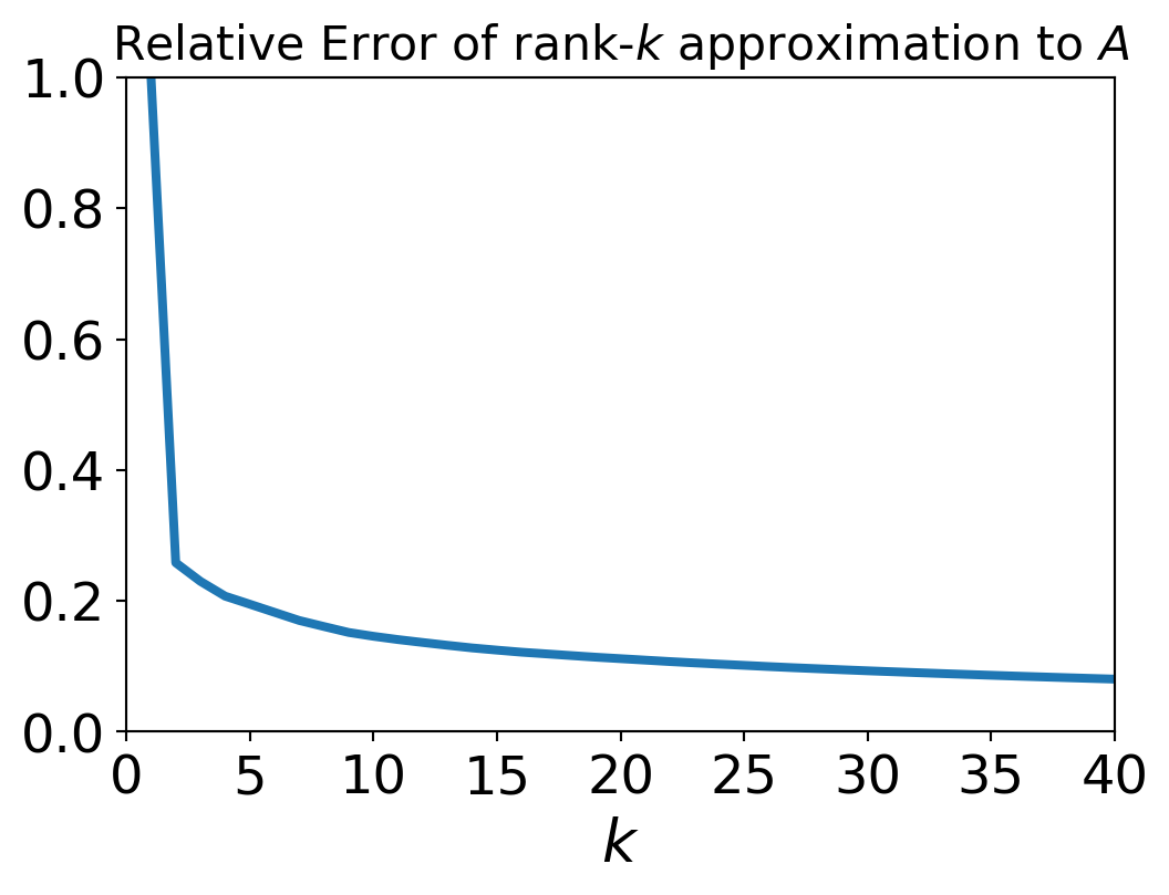
This matrix \(A\) has rank of 512.

But the error when we approximate \(A\) by a rank 40 matrix is only around 10%.

We say that the effective rank of \(A\) is low (perhaps 40).

Let’s find the closest rank-40 matrix to \(A\) and view it.

We can do this quite easily using the SVD.

We simply construct our approximation of \(A\) using only the first 40 columns of \(U\) and top 40 rows of \(V^T\).

\[U\Sigma V^T = A\]

\[A^{(k)} = U'\Sigma'(V')^T.\]

Note that the rank-40 boat takes up only 40/512 = 8% of the space of the original image!

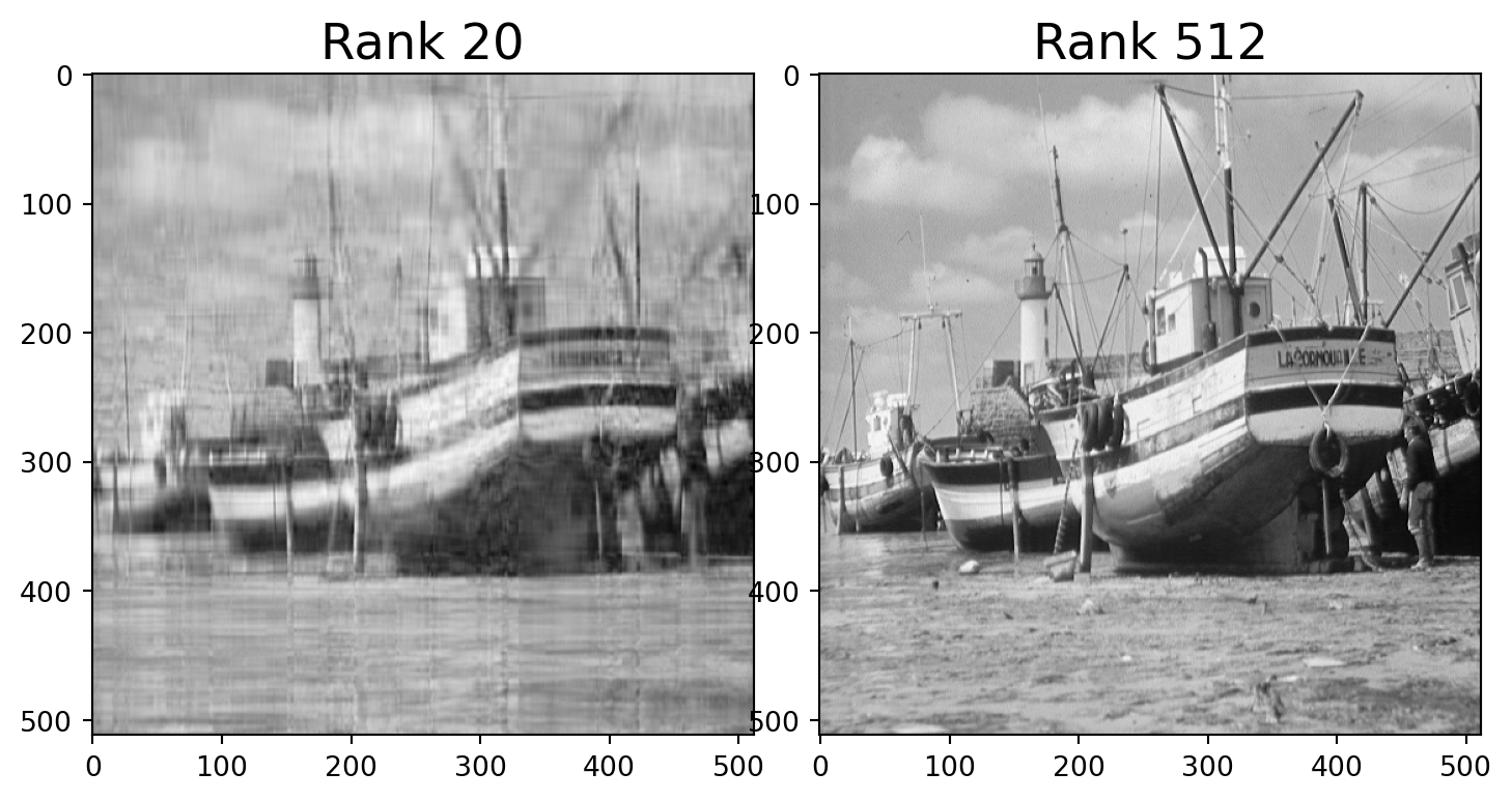
This general principle is what makes image, video, and sound compression effective.

When you

• watch HDTV, or
• listen to an MP3, or
• look at a JPEG image,

these signals have been compressed using the fact that they are effectively low-rank matrices.

As you can see from the example of the boat image, it is often possible to compress such signals enormously, leading to an immense savings of storage space and transmission bandwidth.

In fact the entire premise of the show “Silicon Valley” is based on this fact :)

Dimensionality Reduction

Another way to think about what we just did is “dimensionality reduction”.

Consider this common situation:

\({\text{m objects}}\left\{\begin{array}{c}\;\\\;\\\;\\\;\\\;\end{array}\right.\;\;\overbrace{\left[\begin{array}{ccccc} \begin{array}{c}a_{11}\\\vdots\\a_{i1}\\\vdots\\a_{m1}\end{array}& \begin{array}{c}\dots\\\ddots\\\dots\\\ddots\\\dots\end{array}& \begin{array}{c}a_{1j}\\\vdots\\a_{ij}\\\vdots\\a_{mj}\end{array}& \begin{array}{c}\dots\\\ddots\\\dots\\\ddots\\\dots\end{array}& \begin{array}{c}a_{1n}\\\vdots\\a_{in}\\\vdots\\a_{mn}\end{array} \end{array}\right]}^{\text{n features}} = \overbrace{\left[\begin{array}{ccc}\vdots&&\vdots\\\vdots&&\vdots\\\mathbf{u}_1&\cdots&\mathbf{u}_k\\\vdots&&\vdots\\\vdots&&\vdots\end{array}\right]}^{\large k} \times \left[\begin{array}{ccc}\sigma_1& &\\&\ddots&\\&&\sigma_k\end{array}\right] \times \left[\begin{array}{ccccc}\dots&\dots&\mathbf{v}_1&\dots&\dots\\&&\vdots&&\\\dots&\dots&\mathbf{v}_k&\dots&\dots\end{array}\right]\)

The \(U\) matrix has a row for each data object.

Notice that the original data objects had \(n\) features, but each row of \(U\) only has \(k\) entries.

Despite that, a row of \(U\) can still provide most of the information in the corresponding row of \(A\)

(To see that, note that we can approximately recover the original row by simply multiplying the row of \(U\) by \(\Sigma V^T\)).

So we have reduced the dimension of our data objects – from \(n\) down to \(k\) – without losing much of the information they contain.

Principal Component Analysis

This kind of dimensionality reduction can be done in an optimal way.

The method for doing it is called Principal Component Analysis (or PCA).

What does optimal mean in this context?

Here we use a statistical criterion: a dimensionality reduction that captures the maximum variance in the data.

Here is a simple example.

Consider the points below, which live in \(\mathbb{R}^2\).

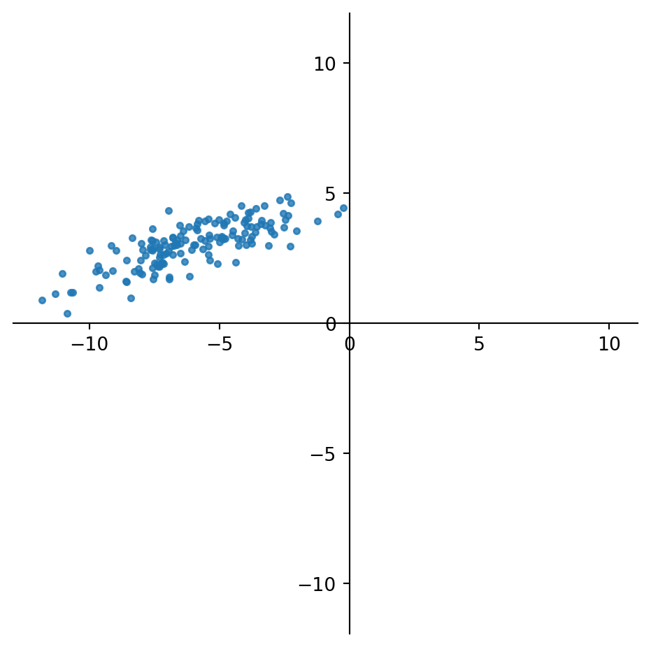
Now, although the points are in \(\mathbb{R}^2\), they seem to show effective low-rank.

That is, it might not be a bad approximation to replace each point by a point in a 1-D dimensional space, that is, along a line.

What line should we choose? We will choose the line such that the sum of the distances of the points to the line is minimized.

The points, projected on this line, will capture the maximum variance in the data (because the remaining errors are minimized).

What would happen if we used SVD at this point, and kept only rank-1 approximation to the data?

This would be the 1-D subspace that approximates the data best in Frobenius norm.

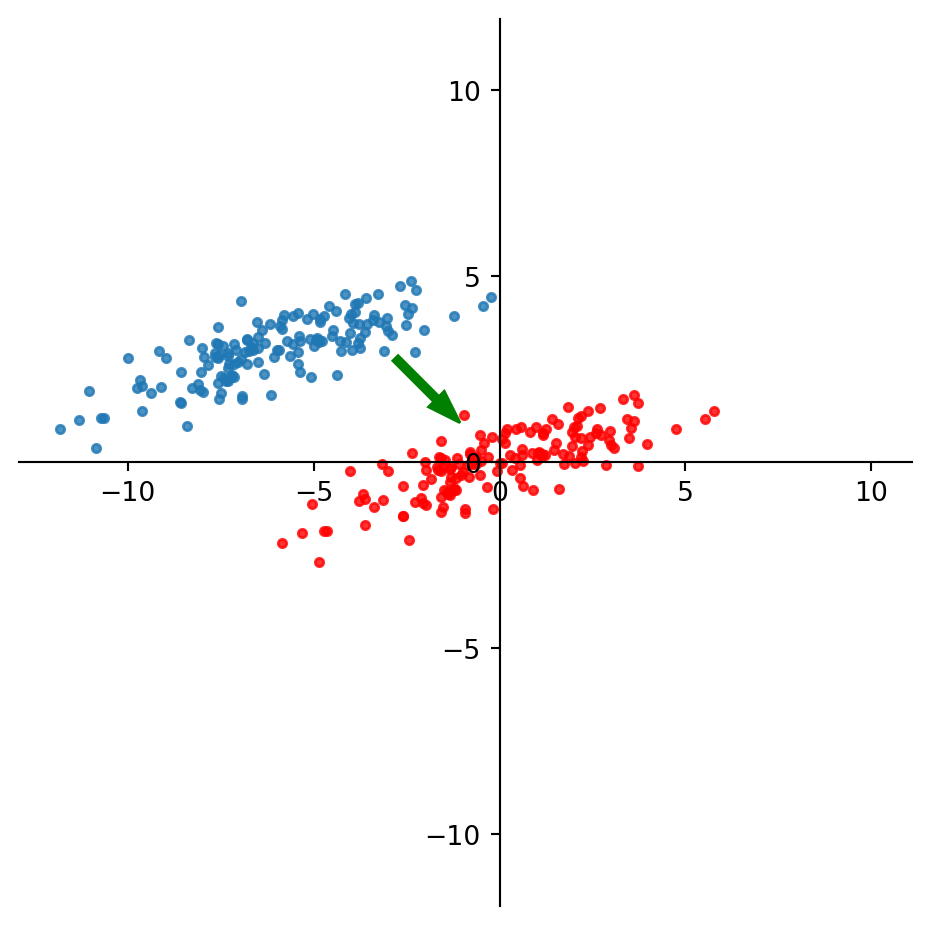
However the variance in the data is defined with respect to the data mean, so we need to mean-center the data first, before using SVD.

That is, without mean centering, SVD finds the best 1-D subspace, not the best line though the data (which might not pass through the origin).

So to capture the best line through the data, we first move the data points to the origin:

Now we use SVD to construct the best 1-D approximation of the mean-centered data:

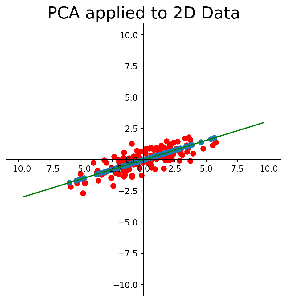
This method is called Principal Component Analysis.

In summary, PCA consists of:

  1. Mean center the data, and

  2. Reduce the dimension of the mean-centered data via SVD.

It winds up constructing the best low dimensional approximation of the data in terms of variance.

This is equivalent to projecting the data onto the subspace that captures the maximum variance in the data.

That is, each point is replaced by a point in \(k\) dimensional space such that the total error (distances between points and their replacements) is minimized.

Visualization using PCA

I’ll now show an extended example to give you a sense of the power of PCA.

Let’s analyze some really high-dimensional data: documents.

A common way to represent documents is using the bag-of-words model.

In this matrix, rows are documents, columns are words, and entries count how many time a word appears in a document.

This is called a document-term matrix.

\[{\text{$m$ documents}}\left\{\begin{array}{c}\;\\\;\\\;\\\;\\\;\end{array}\right.\;\;\overbrace{\left[\begin{array}{ccccc} \begin{array}{c}a_{11}\\\vdots\\a_{i1}\\\vdots\\a_{m1}\end{array}& \begin{array}{c}\dots\\\ddots\\\dots\\\ddots\\\dots\end{array}& \begin{array}{c}a_{1j}\\\vdots\\a_{ij}\\\vdots\\a_{mj}\end{array}& \begin{array}{c}\dots\\\ddots\\\dots\\\ddots\\\dots\end{array}& \begin{array}{c}a_{1n}\\\vdots\\a_{in}\\\vdots\\a_{mn}\end{array} \end{array}\right]}^{\text{$n$ terms}}\]

We are touching on a broad topic, called Latent Semantic Analysis, which is essentially the application of linear algebra to document analysis.

You can learn about Latent Semantic Analysis in other courses in data science or natural language processing.

Our text documents are going to be posts from certain discussion forums called “newsgroups”.

We will collect posts from three groups: comp.os.ms-windows.misc, sci.space, and rec.sport.baseball.

I am going to skip over some details. However, all the code is here, so you can explore it on your own if you like.

from sklearn.datasets import fetch_20newsgroups
categories = ['comp.os.ms-windows.misc', 'sci.space', 'rec.sport.baseball']
news_data = fetch_20newsgroups(subset='train', categories=categories)
from sklearn.feature_extraction.text import TfidfVectorizer
vectorizer = TfidfVectorizer(stop_words='english', min_df=4, max_df=0.8)
dtm = vectorizer.fit_transform(news_data.data).todense()

print('The size of our document-term matrix is {}'.format(dtm.shape))

The size of our document-term matrix is (1781, 9409)

So we have 1781 documents, and there are 9409 different words that are contained in the documents.

We can think of each document as a vector in 9409-dimensional space.

Let us apply PCA to the document-term matrix.

First, we mean center the data.

centered_dtm = dtm - np.mean(dtm, axis=0)

Now we compute the SVD of the mean-centered data:

u, s, vt = np.linalg.svd(centered_dtm)

Now, we use PCA to visualize the set of documents.

Our visualization will be in two dimensions.

This is pretty extreme …

– we are taking points in 9409-dimensional space and projecting them into a subspace of only two dimensions!

Xk = u @ np.diag(s)
fig, ax = plt.subplots(1,1,figsize=(7,6))
plt.scatter(np.ravel(Xk[:,0]), np.ravel(Xk[:,1]), 
                    s=20, alpha=0.5, marker='D')
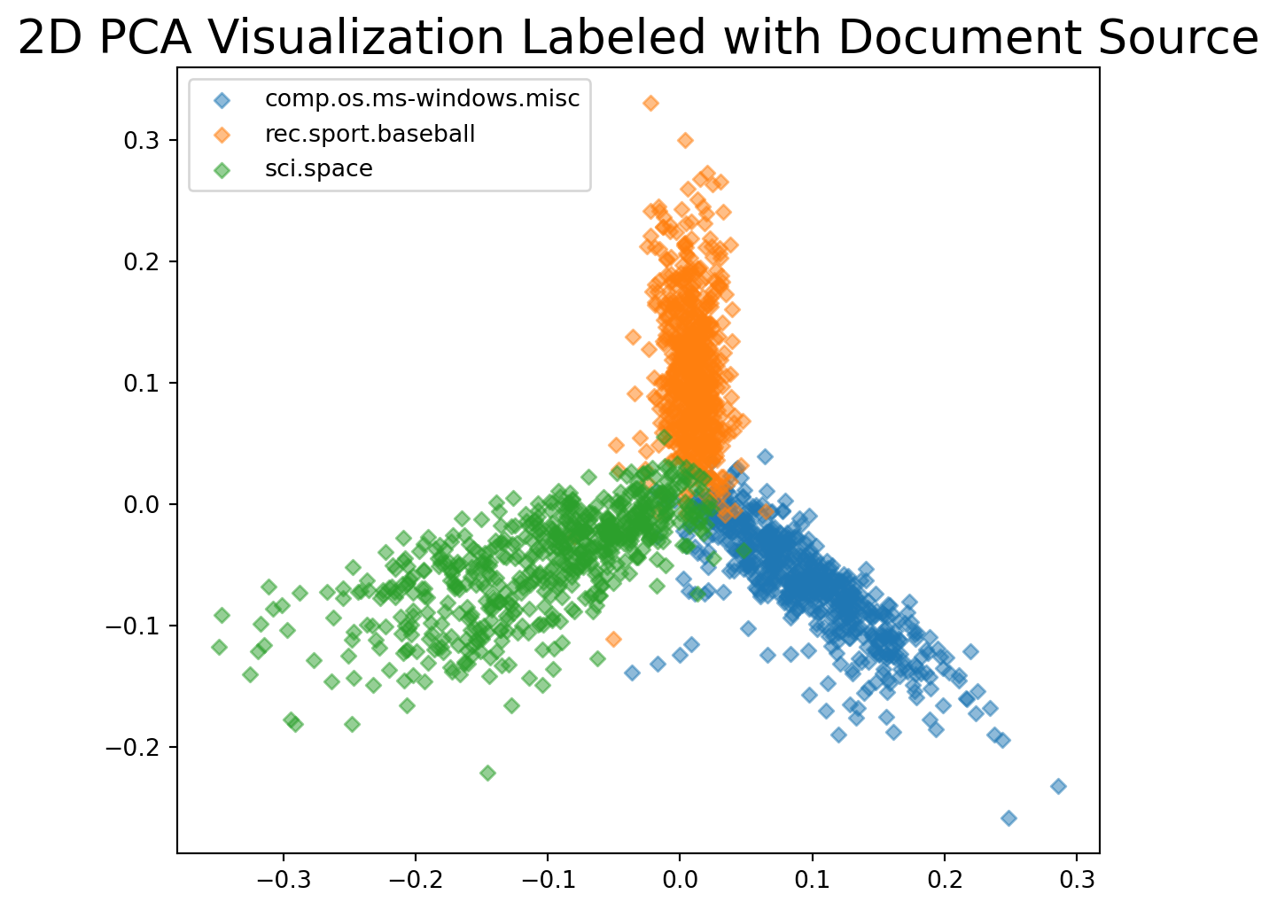
plt.title('2D Visualization of Documents via PCA', size=20);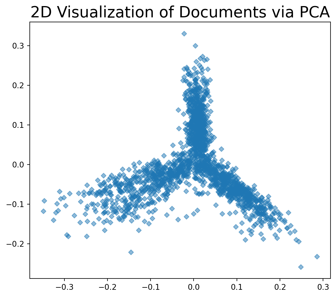

This visualization shows that our collection of documents has considerable internal structure.

In particular, based on word frequency, it appears that there are three general groups of documents.

As you might guess, this is because the discussion topics of the document sets are different:

In summary:

• Data often arrives in high dimension
  • for example, the documents above are points in \(\mathbb{R}^{9049}\)
• However, the structure in data can be relatively low-dimensional
  • in our example, we can see structure in just two dimensions!
• PCA allows us to find the low-dimensional structure in data
  • in a way that is optimal in some sense