Markov was part of the great tradition of mathematics in Russia.
Markov started out working in number theory but then got interested in probability. He enjoyed poetry and the great Russian poet Pushkin. Markov studied the sequence of letters found in the text of Eugene Onegin, in particular the sequence of consonants and vowels.
He sought a way to describe patterns in sequences, such as text like Eugene Onegin. This eventually led to the idea of a system in which one transitions between states, and the probability of going to another state depends only on the current state.
Hence, Markov pioneered the study of systems in which the future state of the system depends only on the present state in a random fashion. This has turned out to be a terrifically useful idea. For example, it is the starting point for analysis of the movement of stock prices, and the dynamics of animal populations.
These have since been termed “Markov Chains.”
Markov chains are essential tools in understanding, explaining, and predicting phenomena in computer science, physics, biology, economics, and finance.
Today we will study an application of linear algebra. You will see how the concepts we use, such as vectors and matrices, get applied to a particular problem.
Many applications in computing are concerned with how a system behaves over time.
Think of a Web server that is processing requests for Web pages, or network that is moving packets from place to place.
We would like to describe how systems like these operate, and analyze them to understand their performance limits.
A typical way to model a time-evolving system is:
define some vector that describes the state of the system, and
formulate a rule that specifies how to compute the next state of the system based on the current state of the system.
So we would say that the state of the system at time \(k\) is a vector \({\bf x_k} \in \mathbb{R}^n,\) and
We can see that this is correct by verifying that:
\[\left[\begin{array}{cc}\text{city pop. in 2001}\\\text{suburb pop. in 2001}\end{array}\right] =\left[\begin{array}{rr}.95&.03\\.05&.97\end{array}\right] \left[\begin{array}{cc}\text{city pop. in 2000}\\\text{suburb pop. in 2000}\end{array}\right].\]
So we think of a probability vector \({\bf x_0}\) as describing how things are “distributed” across various categories – the fraction of items that are in each category.
And we think of the stochastic matrix \(A\) as describing how things “redistribute” themselves at each time step.
Example. Suppose that in 2000 the population of the city is 600,000 and the population of the suburbs is 400,000. What is the distribution of the population in 2001? In 2002? In 2020?
Solution. First, we convert the population counts to a probability vector, in which elements sum to 1.
This is done by simply normalizing by the sum of the vector elements.
Let’s compute the state vectors \({\bf x_1},\dots,{\bf x_{15}}\) to find out.
# stochastic matrix AA = np.array( [[.5, .2, .3], [.3, .8, .3], [.2, 0, .4]])## initial state vectorx = np.array([1,0,0])## array to hold each future state vectorxs = np.zeros((15,3))# # compute future state vectorsfor i inrange(15): xs[i] = xprint(f'x({i}) = {x}') x = A @ x
the sequence of vectors is approaching \(\left[\begin{array}{r}.3\\.6\\.1\end{array}\right]\) as a limit, and
when and if they get to that point, they will stabilize there.
Steady-State Vectors
This convergence to a “steady state” is quite remarkable. Is this a general phenomenon?
Definition. If \(P\) is a stochastic matrix, then a steady-state vector (or equilibrium vector) for \(P\) is a probability vector \(\bf q\) such that:
\[P{\bf q} = {\bf q}.\]
It can be shown that every stochastic matrix has at least one steady-state vector.
(We’ll study this more closely in a later lecture.)
Example.
\(\left[\begin{array}{r}.3\\.6\\.1\end{array}\right]\) is a steady-state vector for \(\left[\begin{array}{rrr}.5&.2&.3\\.3&.8&.3\\.2&0&.4\end{array}\right]\)
The probability vector \({\bf q} = \left[\begin{array}{r}.375\\.625\end{array}\right]\) is a steady-state vector for the population migration matrix \(A\), because
So \(x_1 = \frac{3}{4}x_2\) and \(x_2\) is free. The general solution is \(\left[\begin{array}{c}\frac{3}{4}x_2\\x_2\end{array}\right].\)
This means that there are an infinite set of solutions. Which one are we interested in?
Remember that our vectors \({\bf x}\) are probability vectors. So we are interested in the solution in which the vector elements are nonnegative and sum to 1.
The simple way to find this is to take any solution, and divide it by the sum of the entries (so that the sum then adds to 1.)
Let’s choose \(x_2 = 1\), so the specific solution is:
So, we have found how to solve a Markov Chain for its steady state:
Solve the linear system \((P-I){\bf x} = {\bf 0}.\)
The system will have an infinite number of solutions, with one free variable. Obtain a general solution.
Pick any specific solution (choose any value for the free variable), and normalize it so the entries add up to 1.
Existence of, and Convergence to, Steady State
Finally: when does a system have a unique solution that is a probability vector, and how do we know it will converge to that vector?
Of course, a linear system in general might have no solutions, or it might have a unique solution that is not a probability vector.
So what we are asking is, when does a system defined by a Markov Chain have an infinite set of solutions, so that we can find one of them that is a probability vector?
Definition. We say that a stochastic matrix \(P\) is regular if some matrix power \(P^k\) contains only strictly positive entries.
Since every entry in \(P^2\) is positive, \(P\) is a regular stochastic matrix.
Theorem. If \(P\) is an \(n\times n\) regular stochastic matrix, then \(P\) has a unique steady-state vector \({\bf q}.\) Further, if \({\bf x_0}\) is any initial state and \({\bf x_{k+1}} = P{\bf x_k}\) for \(k = 0, 1, 2,\dots,\) then the Markov Chain \(\{{\bf x_k}\}\) converges to \({\bf q}\) as \(k \rightarrow \infty.\)
Note the phrase “any initial state.”
This is a remarkable property of a Markov Chain: it converges to its steady-state vector no matter what state the chain starts in.
We say that the long-term behavior of the chain has “no memory of the starting state.”
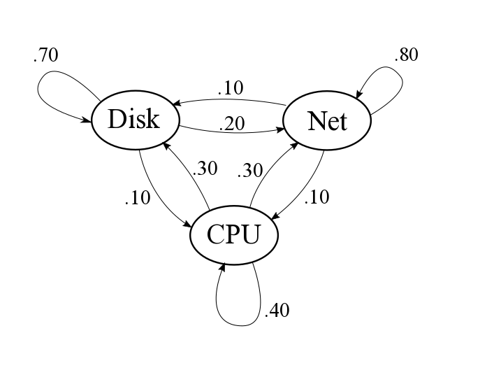
Example. Consider a computer system that consists of a disk, a CPU, and a network interface.
A set of jobs are loaded into the system. Each job makes requests for service from each of the components of the system.
After receiving service, the job then next requests service from the same or a different component, and so on.
Jobs move between system components according to the following diagram.
For example, after receiving service from the Disk, 70% of jobs return to the disk for another unit of service; 20% request service from the network interface; and 10% request service from the CPU.
Assume the system runs for a long time. Determine whether the system will stabilize, and if so, find the fraction of jobs that are using each device once stabilized. Which device is busiest? Least busy?
Solution. From the diagram, the movement of jobs among components is given by:
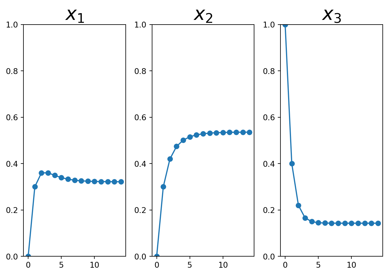
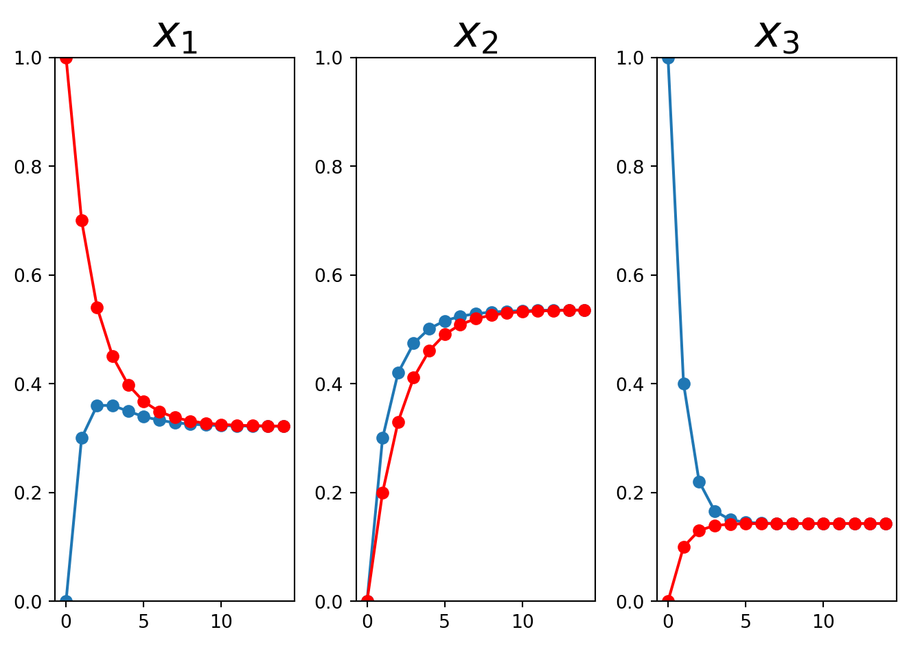
Then let’s look at how the three elements of the \({\bf x}\) vector evolve with time, by computing \(P{\bf x}_0\), \(P^2{\bf x}_0\), \(P^3{\bf x}_0\), etc.
Notice how the system starts in the state \(\left[\begin{array}{r}0\\0\\1\end{array}\right]\),
but quickly (within about 10 steps) reaches the equilibrium state that we predicted:
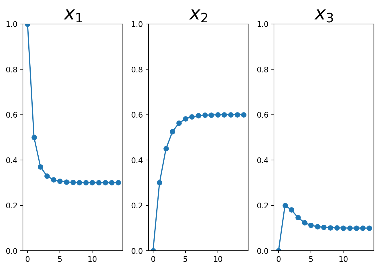
Now let’s compare what happens if the system starts in a different state, say \(\left[\begin{array}{r}1\\0\\0\end{array}\right]\):
This shows graphically that even though the system started in a very different state, it quickly converges to the steady state regardless of the starting state.
Although we have been showing each component converging separately, in fact the entire state vector of the system can be thought of as evolving in space.
This figure shows the movement of the state vector starting from six different initial conditions, and shows how regardless of the starting state, the eventual state is the same.
Summary
Many phenomena can be describe using Markov’s idea:
There are “states”, and
Transition between states only depends on the current state.
Examples: population movement, jobs in a computer, consonants/vowels in a text…
Such a system can be expressed in terms of a stochastic matrix and a probability vector.
Evolution of the system in time is described by matrix multiplication.
Using linear algebraic tools we can predict the steady state of such a system!