p = 0.45
A = np.array([
    [1,   p,   0,   0,   0],
    [0,   0,   p,   0,   0],
    [0, 1-p,   0,   p,   0],
    [0,   0, 1-p,   0,   0],
    [0,   0,   0, 1-p,   1]
])

B = np.linalg.matrix_power(A, 100)

steady_state = B @ np.array([0, 0, 1, 0, 0])PageRank
Larry Page and Sergey Brin
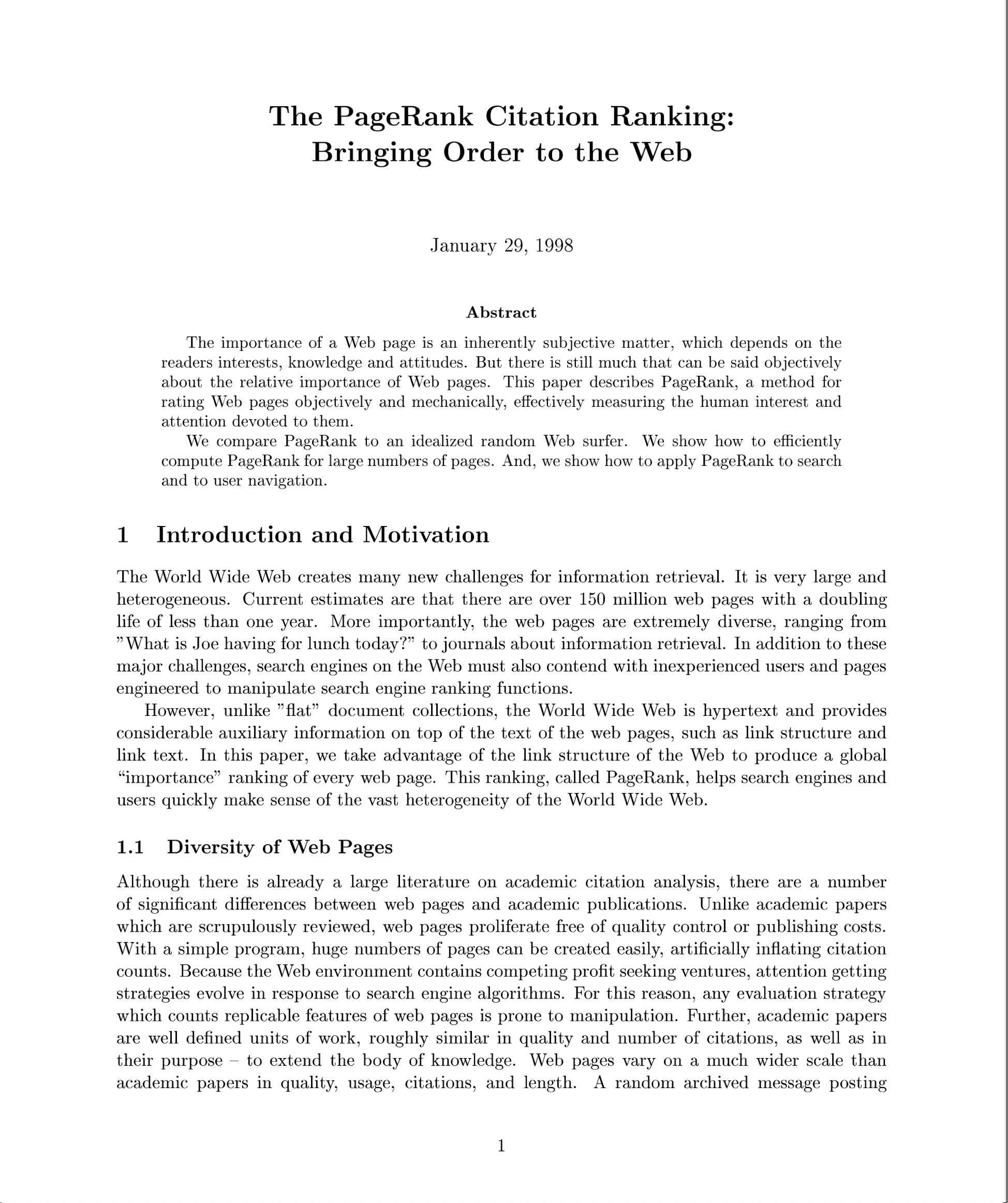
The PageRank paper
The History
Today we’ll study an algorithm that is probably important in your life: Google’s PageRank.
Many parts of this page are based on Linear Algebra and its Applications, by David C. Lay
Let’s set the stage.
The World Wide Web started becoming widely used in 1994.
By 1998 the Web had become an indispensable information resource.
However, the problem of effectively searching the Web for relevant information was not well addressed. A number of large search engines were available, with names that are now forgotten: Alta Vista, Lycos, Excite, and others.
At present, most of them are no longer in existence, because Google emerged in 1998 and came to dominate Web search almost overnight.
How did this happen?
As background: a typical search engine uses a two-step process to retrieve pages related to a user’s query.
In the first step, basic text processing is done to find all documents that contain the query terms. Due to the massive size of the Web, this first step can result in thousands to millions of retrieved pages related to the query.
Some of these pages are important, but most are not.
The problem that Google solved better than it competitors is deciding the ordering in which the resulting search results are presented. This is crucial: a user wants to find the “correct” or “best” item at the top of the search results.
By displaying the most relevant pages at the top of the list returned each query, Google makes its search results very useful. The algorithm that gave Google this advantage is called PageRank.
The Insight
Around 1998, the limitations of standard search engines, which just used term frequency, we becoming apparent. A number of researchers were thinking about using additional sources of information to “rate” pages.
The key idea that a number of researchers hit on was this: links are endorsements.
When a first page contains a link to a second page, that is an indication that the author of the first page thinks the second page is worth looking at. If the first and second pages both contain the same query terms, it is likely that the second page is an important page with respect to that query term.
Consider a set of web pages, for a single query term (say “car manufacturers”) with this linking structure:
It may be clear that the links between pages contain useful information. But what is the best way to extract that information in the form of rankings?
Here is the strategy that Brin and Page used:
From “The anatomy of a large-scale hypertextual Web search engine” (1998):
Today we’ll study this algorithm, see how to implement it, and understand that what it is really about is Markov Chains and eigenvectors.
Random Walks
We start with the notion of a random walk.
A random walk is a model of many sorts of processes that occur on graphs.
Let us fix a graph \(G\). A random walk models the movement of an object on this graph.
We assume that the object moves from node to node in \(G\), one move per time step \(t.\) At time \(t\) the object is at node \(k\) (say) and at the next time \(t+1\) it moves to another node chosen at random from among the outgoing edges.
For our initial discussion, we will assume that \(G\) is the line graph:
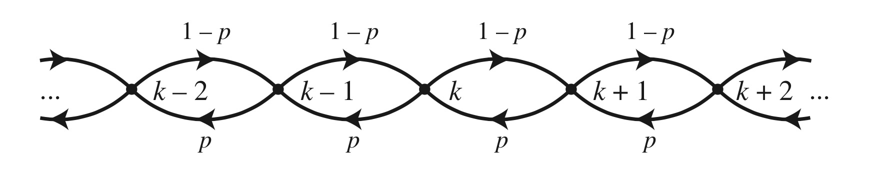
This is a graph in which each node is connected to two neighbors. It’s natural to identify the nodes with the integers \(k = 1,\dots,n.\)
An example application of this model would be a waiting line (or ‘queue’) like at a grocery store. The current node corresponds to the number of people in the queue. Given some number of people in the queue, only one of two things happens: either a person leaves the queue or a person joins the queue.
In fact, this sort of model is used for jobs running in a CPU – it is studied in CS350.
To complete the definition, what happens at the endpoints of the graph (nodes 1 and \(n\)) must be specified.
One possibility is for the walker to remain fixed at that location. This is called a random walk with absorbing boundaries.
Another possibility is for the walker to bounce back one unit when an endpoint is reached. This is called a random walk with reflecting boundaries.
We can also set a particular probability \(1-p\) of moving “to the right” (from \(k\) to \(k+1\)) and \(p\) of moving “to the left” (from \(k\) to \(k-1\)).
Now, here is a cool idea:
We can describe a random walk on \(G\) as a Markov chain.
The way to interpret the steady-state of the Markov chain in terms of the random walk is:
Let the chain (random walk) start in the given state. At some long time in the future, make an observation of the state that the chain is in. Then the steady-state distribution gives, for each state, the probability that the chain is in that state when we make our observation.
As a reminder, recall these facts about a Markov Chain.
For a Markov Chain having transition matrix \(P\):
- The largest eigenvalue of \(P\) is 1.
- If \(P\) is regular, then
- There is only one eigenvalue equal to 1
- The chain will converge to the corresponding eigenvector as its unique steady-state.
- “\(P\) is regular” means that for some \(k>0\), all entries in \(P^k\) are nonzero.
Absorbing Boundaries
Example. A random walk on \(\{0,1,2,3,4\}\) with absorbing boundaries has a transition matrix of
\[P=\begin{bmatrix}1&p&0&0&0\\0&0&p&0&0\\0&1-p&0&p&0\\0&0&1-p&0&0\\0&0&0&1-p&1\end{bmatrix}\]
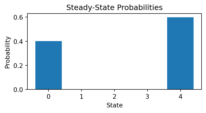
Example. (“Gambler’s Ruin”). Consider a very simple casino game. A gambler (with some money to lose) flips a coin and calls heads or tails. If the gambler is correct, she wins a dollar. If she is wrong, she loses a dollar. The gambler will quit the game when she has either won \(n-1\) dollars or lost all of her money.
Suppose that \(n=5\) and the gambler starts with $2. The gambler’s winnings must move up or down one dollar with each coin flip, and once the gambler’s winnings reach 0 or 4, they do not change any more since the gambler has quit the game.
Such a process may be modeled as a random walk on \(\{0,1,2,3,4\}\) with absorbing boundaries. Since a move up or down is equally likely in this case, \(p = 1/2\).
This transition matrix is not regular. Why? Consider column 1.
There is not a unique steady-state to which the chain surely converges.
However, it turns out there are two long-term possibilities for the walker, each corresponding to absorption at one boundary, and the walker will surely get stuck at one or the other.
In other words, in this case, there are two different eigenvectors corresponding to the eigenvalue 1. So the dimension of this eigenspace is two.
In terms of our problem, this means that the gambler eventually either wins or loses (as opposed to going up and down for an arbitrarily long time).
Using slightly more advanced methods, we can predict the probabilities of landing in one steady-state or the other.
For example, if \(p=0.45\), we find that the probability that the gambler will lose all her money to be \(0.4\).
Random Walks on Undirected Graphs
Now let’s consider a random walk on a more interesting graph:
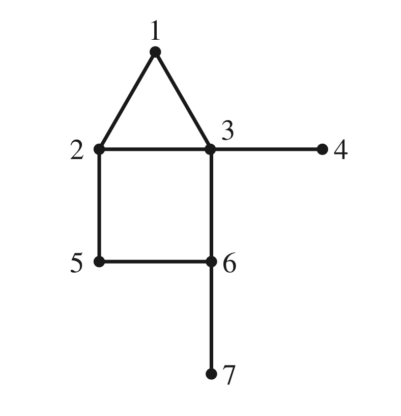
This graph is undirected – each edge can be followed in either direction.
Again, at each node there is an equal probability of departing to any adjacent node.
The transition matrix associated with a random walk on this graph is
\[P = \begin{bmatrix} 0&1/3&1/4&0&0&0&0\\ 1/2&0&1/4&0&1/2&0&0\\ 1/2&1/3&0&1&0&1/3&0\\ 0&0&1/4&0&0&0&0\\ 0&1/3&0&0&0&1/3&0\\ 0&0&1/4&0&1/2&0&1\\ 0&0&0&0&0&1/3&0\end{bmatrix}\]
It turns out that this matrix is regular (\(P^3\) has no zero entries.)
Hence, the associated Markov Chain converges to a single steady state.
The eigenvector corresponding to the eigenvalue of 1 is the steady-state of the Markov Chain.
Hence we can find that the steady-state is \(\frac{1}{16}\begin{bmatrix}2\\3\\4\\1\\2\\3\\1\end{bmatrix}.\)
That is, the probability of bring in node 1 at steady state is 2/16; the probability of being in node 2 is 3/16; the probability of being in node 3 is 4/16, etc.
Now, look at \(G\) again, and compare it to its steady-state distribution. Notice anything?
\[\frac{1}{16}\begin{bmatrix}2\\3\\4\\1\\2\\3\\1\end{bmatrix}\]
The steady-state distribution is proportional to the number of edges attached to the node.
The number of edges connected to a node is called the node degree.
This is not a coincidence!
In fact it can be proved that the steady-state distribution of a random walk on an undirected graph is proportional to node degree.
That is, the probability of being at a particular node at steady state is proportional to that node’s degree.
This is really amazing!
Random Walks on Directed Graphs
More interesting behavior arises when we walk randomly on a directed graph.
In this graph, all edges are “one-way streets” – nodes are joined not by lines but by arrows. The chain can move from vertex to vertex, but only in the directions allowed by the arrows.
An example of a directed graph is
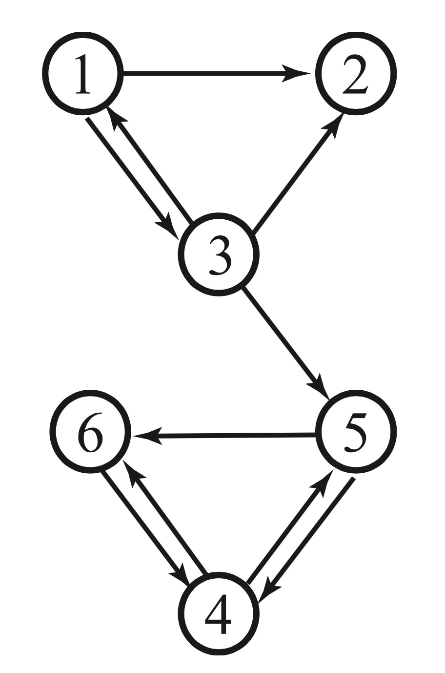
The transition matrix for this graph is:
\[P = \begin{bmatrix} 0&0&1/3&0&0&0\\ 1/2&0&1/3&0&0&0\\ 1/2&0&0&0&0&0\\ 0&0&0&0&1/2&1\\ 0&0&1/3&1/2&0&0\\ 0&0&0&1/2&1/2&0 \end{bmatrix}\]
We can conclude that this matrix is not regular. Why?
One reason we can conclude this is the column of zeros (column 2).
Any power of \(P\) will preserve this column of zeros.
PageRank
There are many ways to use link structure to infer which pages are most important.
There was a lot of experimentation in the late 1990s with various methods.
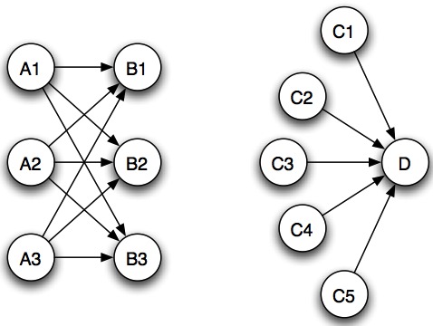
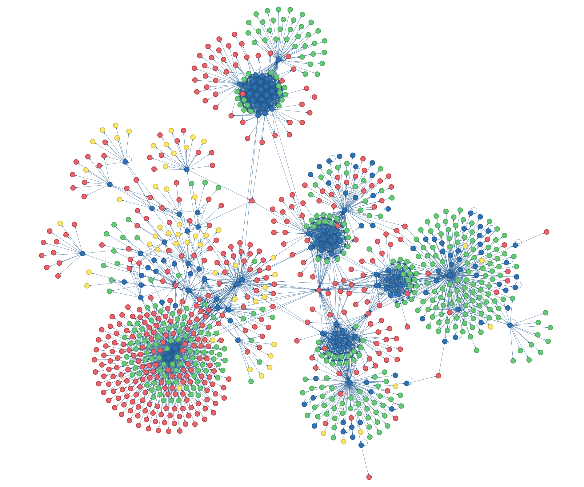
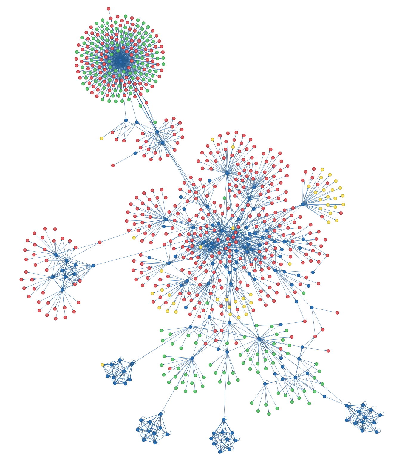
Here are some examples of link structures found in the Web.
Each node is a Web page, and each edge is a link from one Web page to another.
Why did Page and Brin settle on the random walk as the basis for their approach?
In fact, the intuiution they started from was simpler:
Their insight was just to say that a page is ‘important’ if many ‘important’ pages link to it.
More precisely, this definition of ‘importance’ is:
\[\small\text{Importance of page $i$} = \\ \sum_j \text{(Importance of page $j$)}\cdot\text{(Probability of going from page $j$ to page $i$.)}\]
This is a very intuitive definition of importance.
There is a bit of a issue however – it is self-referential!
The ‘importance’ of a page appears on both sides of the equation.
How can we solve this equation to get a fixed ‘importance’ for a given page?
Answering this question is where the random walk comes in.
Let’s define a vector \(\mathbf{x}\) to hold importance:
\[ \mathbf{x} = \begin{bmatrix}\text{importance of page 1}\\\text{importance of page 2}\\\vdots\\\text{importance of page n}\end{bmatrix} \]
And let’s define \(P\) as the transition matrix of the Markov Chain defined by the link structure of the pages:
\[ P_{ij} = \text{probability of going from page } j \text{ to page } i \text{ in a random walk}\]
What Page and Brin observed was that this equation
\[\small\text{Importance of page $i$} = \] \[ \sum_j \text{(Importance of page $j$)}\cdot\text{(Probability of going from page $j$ to page $i$.)}\]
is the same as:
\[\mathbf{x} = P\mathbf{x}\]
Which is the equation defining the steady state of the Markov chain \(P\).
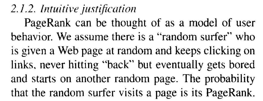
Now we are ready to understand what Page and Brin were saying in 1998:
PageRank can be thought of as a model of user behavior. We assume there is a “random surfer” who is given a web page at random and keeps clicking on links, never hitting “back” but eventually gets bored and starts on another random page. The probability that the random surfer visits a page is its PageRank.
What they are implying is that a random surfer should visit important pages more often and unimportant pages less often.
The way to interpret this precisely is:
1. Form the graph that encodes the connections between Web pages that are retrieved for a particular query.
2. Construct a Markov chain that corresponds to a random walk on this graph.
3. Rank-order the pages according to their probability in the Markov chain’s steady state.
There is a nice visualization here.
So let’s try to make this work and see what happens.
Example.
Assume a set of Web pages have been selected based on a text query, eg, pages related to “personal 737 jets.”
These pages have various links between them, as represented by this graph:
Let’s construct the unique steady-state distribution for a random walk on this graph, if it exists. That is, we will construct the PageRank for this set of Web pages.
The key question we must ask is whether a unique steady state exists.
Step 1.
Assume there are \(n\) pages to be ranked. Construct an \(n\times n\) transition matrix for the Markov chain.
Set the Markov chain transitions so that each outgoing link from a node has equal probability of being taken.
We have already seen the transition matrix for this graph:
\[P = \begin{bmatrix} 0&0&1/3&0&0&0\\ 1/2&0&1/3&0&0&0\\ 1/2&0&0&0&0&0\\ 0&0&0&0&1/2&1\\ 0&0&1/3&1/2&0&0\\ 0&0&0&1/2&1/2&0 \end{bmatrix}\]
We have observed that this transition matrix is not regular, because for any \(P^k, k>0,\) the second column will be zero.
To address this, let’s ask why it happens.
The reason that column 2 of \(P\) is zero is that the Web page corresponding to node 2 has no links embedded in it, so there is nowhere to go from this page. Of course this will happen a lot in an arbitrary collection of Web pages.
Note that Page and Brin say that the random surfer will occasionally “start on another random page.” In other words, it seems reasonable that when reaching a page with no embedded links, the surfer chooses another page at random.
So this motivates the first adjustment to \(P\):
Step 2.
Form the matrix \(P'\) as follows: for each column in \(P\) that is entirely zeros, replace it with a column in which each entry is \(1/n\).
In our example:
\[\tiny P = \begin{bmatrix} 0&0&1/3&0&0&0\\ 1/2&0&1/3&0&0&0\\ 1/2&0&0&0&0&0\\ 0&0&0&0&1/2&1\\ 0&0&1/3&1/2&0&0\\ 0&0&0&1/2&1/2&0 \end{bmatrix} \;\;{\rightarrow}\;\; P' = \begin{bmatrix} 0&1/n&1/3&0&0&0\\ 1/2&1/n&1/3&0&0&0\\ 1/2&1/n&0&0&0&0\\ 0&1/n&0&0&1/2&1\\ 0&1/n&1/3&1/2&0&0\\ 0&1/n&0&1/2&1/2&0 \end{bmatrix}\;\;=\;\; \begin{bmatrix} 0&1/6&1/3&0&0&0\\ 1/2&1/6&1/3&0&0&0\\ 1/2&1/6&0&0&0&0\\ 0&1/6&0&0&1/2&1\\ 0&1/6&1/3&1/2&0&0\\ 0&1/6&0&1/2&1/2&0 \end{bmatrix}\]
Nonetheless, even after this change, \(P'\) can fail to be regular.
In other words, for an arbitrary set of web pages, there is no guarantee that their transition matrix will be regular.
Once again, let’s read the words of Page and Brin closely: the surfer “eventually gets bored and starts on another random page.”
Step 3.
In practice this means that there a small probability that the surfer will jump from any page to any other page at random.
Let’s call this small probability \(\alpha.\)
We can’t just add \(\alpha\) to every entry in \(P'\), because then the columns of the new matrix would not sum to 1.
Instead we decrease each entry in \(P'\) by a factor of \((1-\alpha)\), and then add \({\alpha}/{n}\) to it.
So we compute the final transition matrix \(P''\) as:
\[P''_{ij} = (1-\alpha)P'_{ij} + \frac{\alpha}{n}.\]
We can write this as a matrix equation:
\[P'' = (1-\alpha)P' + \frac{\alpha}{n} \mathbf{1}\]
where \(\mathbf{1}\) is an \(n\times n\) matrix of 1’s.
In our example, let’s say that \(\alpha = 1/10\) (in reality it would be smaller). So \(\alpha/n = 1/60.\)
Then:
\[ \tiny P' \begin{bmatrix} 0&1/6&1/3&0&0&0\\ 1/2&1/6&1/3&0&0&0\\ 1/2&1/6&0&0&0&0\\ 0&1/6&0&0&1/2&1\\ 0&1/6&1/3&1/2&0&0\\ 0&1/6&0&1/2&1/2&0 \end{bmatrix} \;\;{\rightarrow}\;\; P'' = \begin{bmatrix} 1/60&1/6&19/60&1/60&1/60&1/60\\ 7/15&1/6&19/60&1/60&1/60&1/60\\ 7/15&1/6&1/60&1/60&1/60&1/60\\ 1/60&1/6&1/60&1/60&7/15&11/12\\ 1/60&1/6&19/60&7/15&1/60&1/60\\ 1/60&1/6&1/60&7/15&7/15&1/60 \end{bmatrix}\]
Obviously, \(P''\) is regular, because all its entries are positive (they are at least \(\alpha/n.\))
\(P''\) is the Markov Chain that Brin and Page defined, and which is used by PageRank to rank pages in response to a Google search.
Step 4.
Compute the steady-state of \(P''\), and rank pages according to their magnitude in the resulting vector.
We can do this by solving \(P''\mathbf{x} = \mathbf{x}\), or we can compute the eigenvectors of \(P''\) and use the eigenvector that corresponds to \(\lambda = 1.\)
For the example \(P''\), we find that the steady-state vector is:
\(\mathbf{x} = \begin{bmatrix}0.037\\0.054\\0.041\\0.375\\0.206\\0.286\end{bmatrix}\)
So the final ranking of pages is: 4, 6, 5, 2, 3, 1.
This is the order that PageRank would display its results, with page 4 at the top of the list.
Let’s see how to do Step 4 in Python:
# Here is the P'' matrix as computed in steps 1 through 3.
P = np.array([
[1./60, 1./6, 19./60, 1./60, 1./60,  1./60],
[7./15, 1./6, 19./60, 1./60, 1./60,  1./60],
[7./15, 1./6,  1./60, 1./60, 1./60,  1./60],
[1./60, 1./6,  1./60, 1./60, 7./15, 11./12],
[1./60, 1./6, 19./60, 7./15, 1./60,  1./60],
[1./60, 1./6,  1./60, 7./15, 7./15,  1./60]
])
eigenvalues, eigenvectors = np.linalg.eig(P)
print(np.real(eigenvalues))
[ 1. 0.61008601 -0.08958752 -0.37049849 -0.45 -0.45 ]# find the location of the largest eigenvalue (1),
# by computing the indices that would sort the eigenvalues
# from smallest to largest
indices = np.argsort(eigenvalues)
# and take the index of the largest eigenvalue
principal = indices[-1]
print(principal)0# using the index of the largest eigenvalue, extract
# the corresponding eigenvector (the steady state vector)
steadyState = np.real(eigenvectors[:,principal])
steadyState = steadyState/np.sum(steadyState)
print(steadyState)[0.03721197 0.05395735 0.04150565 0.37508082 0.20599833 0.28624589]# find the order of the pages in the steady state vector
# this function sorts from smallest to largest (reverse of what we want)
reverseOrder = np.argsort(steadyState)
print(reverseOrder)[0 2 1 4 5 3]# reverse the order to get the most important page first
# and add one to convert from zero indexing to indexing of example
order = 1 + reverseOrder[::-1]
print('final order = {}'.format(order))
print('importance = {}'.format(steadyState[order-1]))final order = [4 6 5 2 3 1]
importance = [0.37508082 0.28624589 0.20599833 0.05395735 0.04150565 0.03721197]
Computing PageRank: the Power Method
From a mathematical standpoint, we are done!
However, from a Computer Science standpoint, there are still some issues.
The most significant issue is simply this: PageRank results must be provided very quickly. Search engines are in competition and speed is a competitive advantage.
Here is an example Google search:
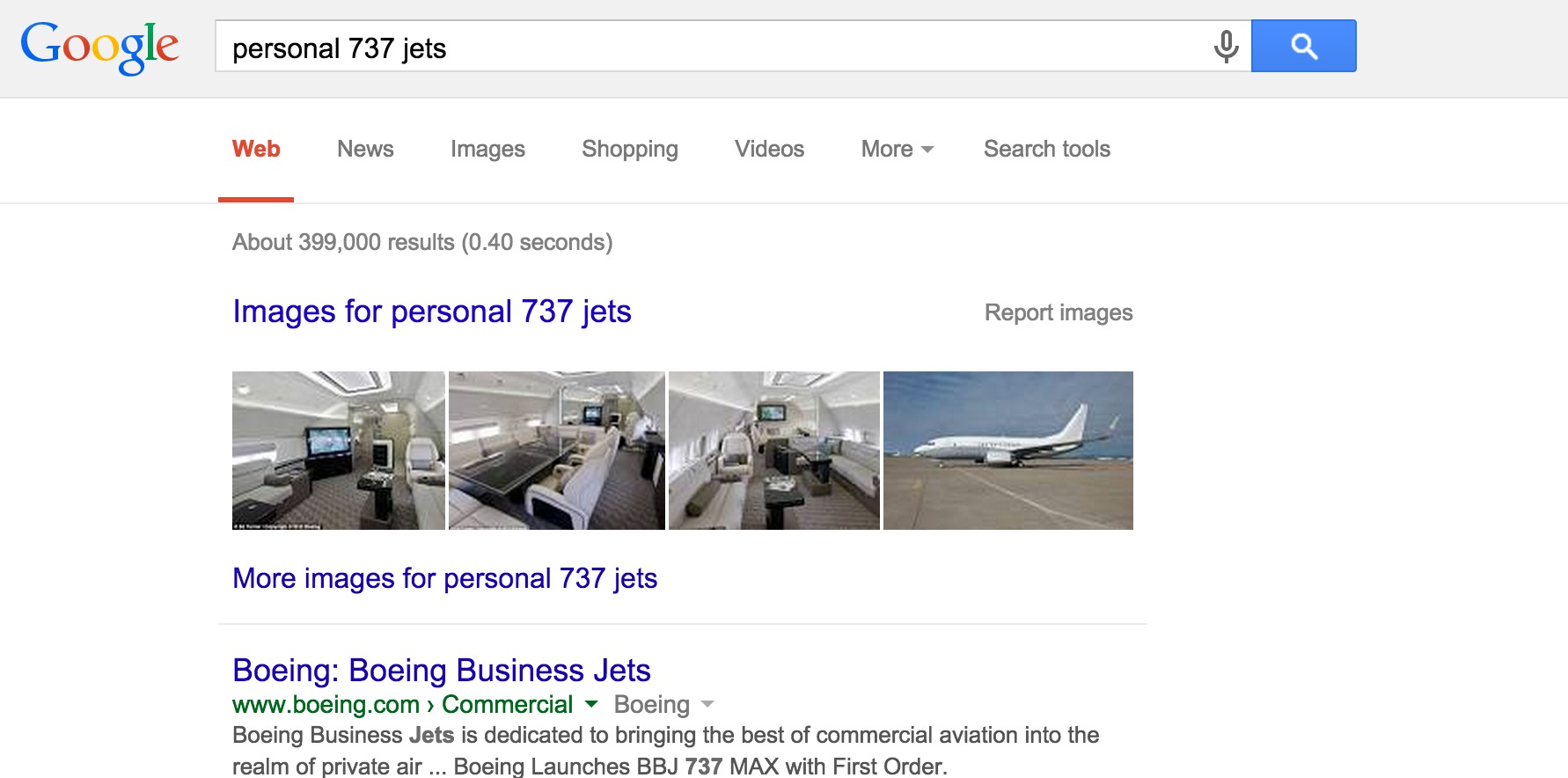
Notice that the search returned about 400,000 results!
Recall that using Gaussian elimination to solve \(A\mathbf{x} = \mathbf{b}\) takes \(\sim \frac{2}{3}n^3\) operations.
In this case, apparently \(n = 400,000.\)
So computing the PageRank in the straightforward way we’ve described would take about 42,667,000,000,000,000 operations.
Assuming a 2GHz CPU, that’s on the order of eight months.
((2./3)*(400000**3))/((2*10**9)*(3600*24*30))8.23045267489712We need a faster way to compute the PageRank!
Here is an important insight: we only need the principal eigenvector. (The one corresponding to \(\lambda = 1\)).
Let’s review how a Markov chain gets to steady state. As we discussed at the end of the lecture on the characteristic equation, the state of the chain at any step \(k\) is given by
\[{\bf x_k} = c_1{\bf v_1}\lambda_1^k + c_2{\bf v_2}\lambda_2^k + \dots + c_n{\bf v_n}\lambda_n^k.\]
Let’s assume that \(\lambda_1\) is the eigenvalue 1. If the chain converges to steady sate, then we know that all eigenvalues other than \(\lambda_1\) are less than 1 in magnitude.
Of course, if \(|\lambda_i| < 1,\)
\[\lim_{k\rightarrow\infty} \lambda_i^k = 0.\]
So:
\[\lim_{k\rightarrow\infty}{\bf x_k} = c_1{\bf v_1}.\]
Note that \(c_1\) is just a constant that doesn’t affect the relative sizes of the components of \({\mathbf{x}_k}\) in the limit of large \(k.\)
This is another way of stating that the Markov chain goes to steady state no matter what the starting state is.
This observation suggests another way to compute the steady state of the chain:
- Start from a random state \(\mathbf{x}_0\).
- Compute \(\mathbf{x}_{k+1} = A\mathbf{x}_k\) for \(k = 0,1,2,3,\dots\)
How do we know when to stop in Step 2?
Since we are looking for steady-state, we can stop when the difference between \(\mathbf{x}_{k+1}\) and \(\mathbf{x}_k\) is small.
This is called the power method.
Why is this a better method?
Keep in mind that the number of flops in matrix-vector multiplication is \(\sim 2n^2\).
This is compared to \(\sim \frac{2}{3}n^3\) for solving the system (finding the eigenvector directly).
Let’s say that after computing
\[\mathbf{x}_1 = A \mathbf{x}_0\]
\[\mathbf{x}_2 = A \mathbf{x}_1\]
\[\mathbf{x}_3 = A \mathbf{x}_2\]
\[\mathbf{x}_4 = A \mathbf{x}_3\]
\[\mathbf{x}_5 = A \mathbf{x}_4\]
\[\mathbf{x}_6 = A \mathbf{x}_5\]
\[\mathbf{x}_7 = A \mathbf{x}_6\]
\[\mathbf{x}_8 = A \mathbf{x}_7\]
\[\mathbf{x}_9 = A \mathbf{x}_8\]
\[\mathbf{x}_{10} = A \mathbf{x}_9\]
we find that \(\mathbf{x}_{10}\) is sufficiently close to \(\mathbf{x}_9.\)
How much work did we do?
We did 10 matrix-vector multiplications, or \(20n^2\) flops.
So the power method is
\[\frac{\frac{2}{3}n^3}{20n^2} = \frac{n}{30}\]
times faster than the direct method.
For our example, \(n/30 = 13,333\). So this trick reduces the running time from 8 months down to 27 minutes.
20*400000.**2/((2*10**9)*(60))26.666666666666668This is an example of an iterative method. Iterative methods are often the preferred approach for solving linear algebra problems in the real world.
One final thing: how exactly do we decide when to stop iterating in the power method?
One simple way is to add up the differences of the components of \(\mathbf{x}_{k+1}-\mathbf{x}_k\):
\[ s = \sum_{i=1}^n |\mathbf{x}_{k+1,i} - \mathbf{x}_{k,i}| \]
and compare it to the sum of the components of \(\mathbf{x}_k\):
\[ d = \sum_{i=1}^n |\mathbf{x}_{k,i}| \]
If \(s/d\) is small (say, less than 0.001) then we can conclude that \(\mathbf{x}_{k+1}\) is close enough to \(\mathbf{x}_k\) for us to stop iterating.
So the power method is fast, making it the algorithm of choice for a company like Google. It is also easy to implement, and easy to parallelize across multiple machines.