Computer Graphics
Many parts of this page are based on Linear Algebra and its Applications, by David C. Lay
Computer Graphics is the study of creating, synthesizing, manipulating, and using visual information in the computer.
Today we’ll study the mathematics behind computer graphics.
If you are interested in learning more about computer graphics, you can take CS 480 here at BU. A good book for more detail specifically on mathematical aspects is Mathematics for 3D Game Programming and Computer Graphics, by Eric Lengyel.
Computer Graphics is Everywhere
Computer graphics (CG) is pervasive in the world today.
Image credits: CS 184 Lecture Slides, UC Berkeley, Ng Ren
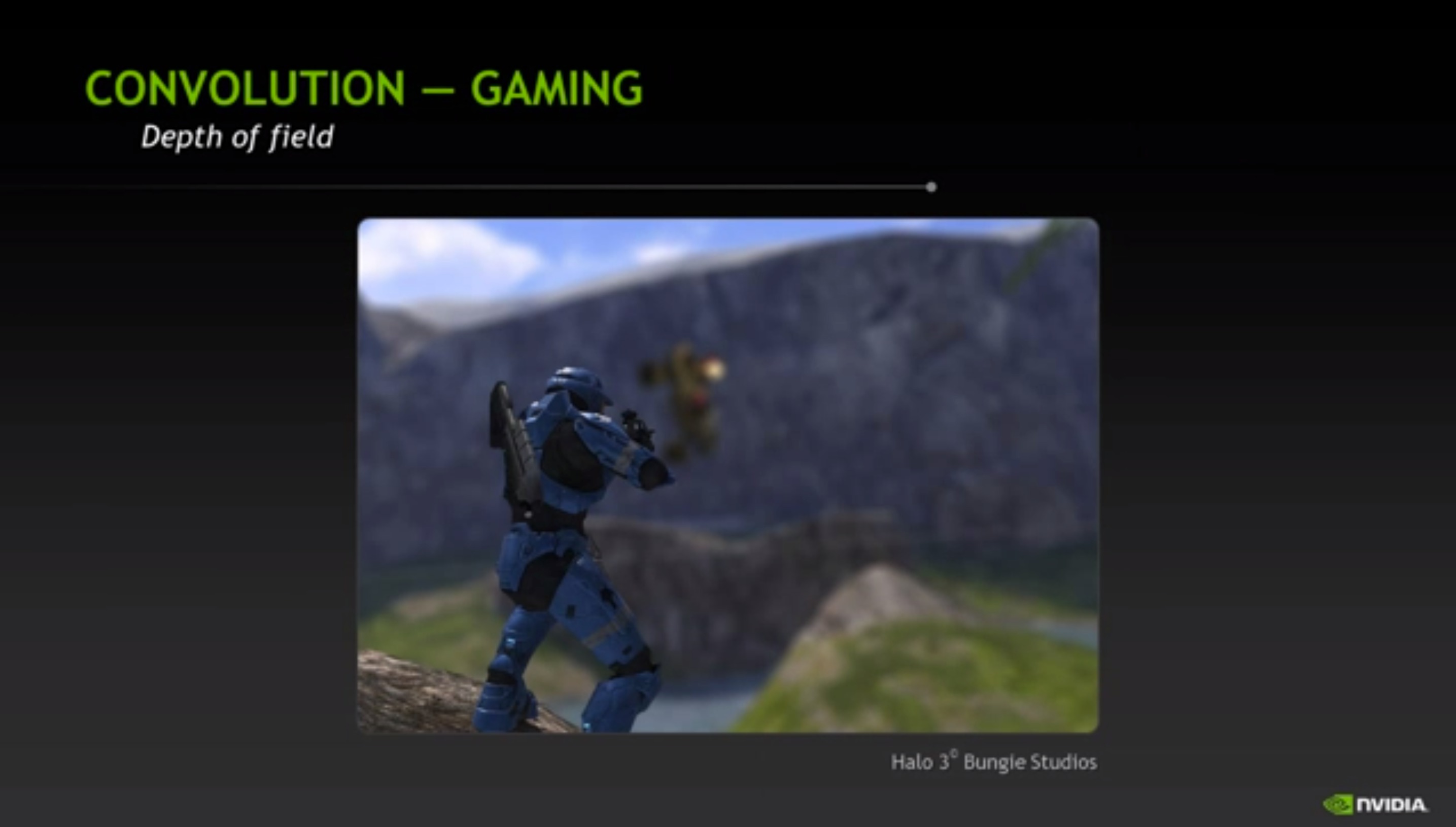
CG is used in films and games.
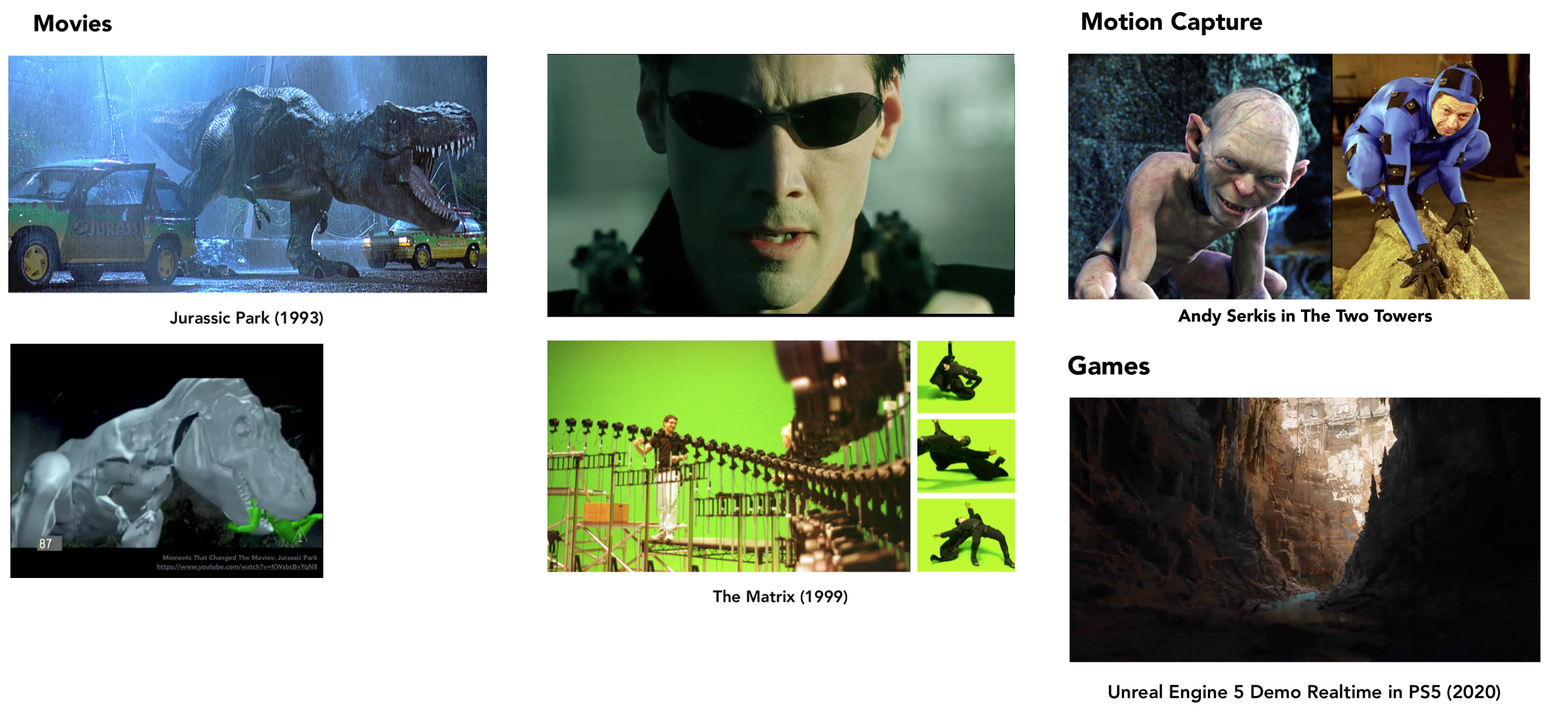
CG is used in science and engineering for product design, visualization and computer-aided design.
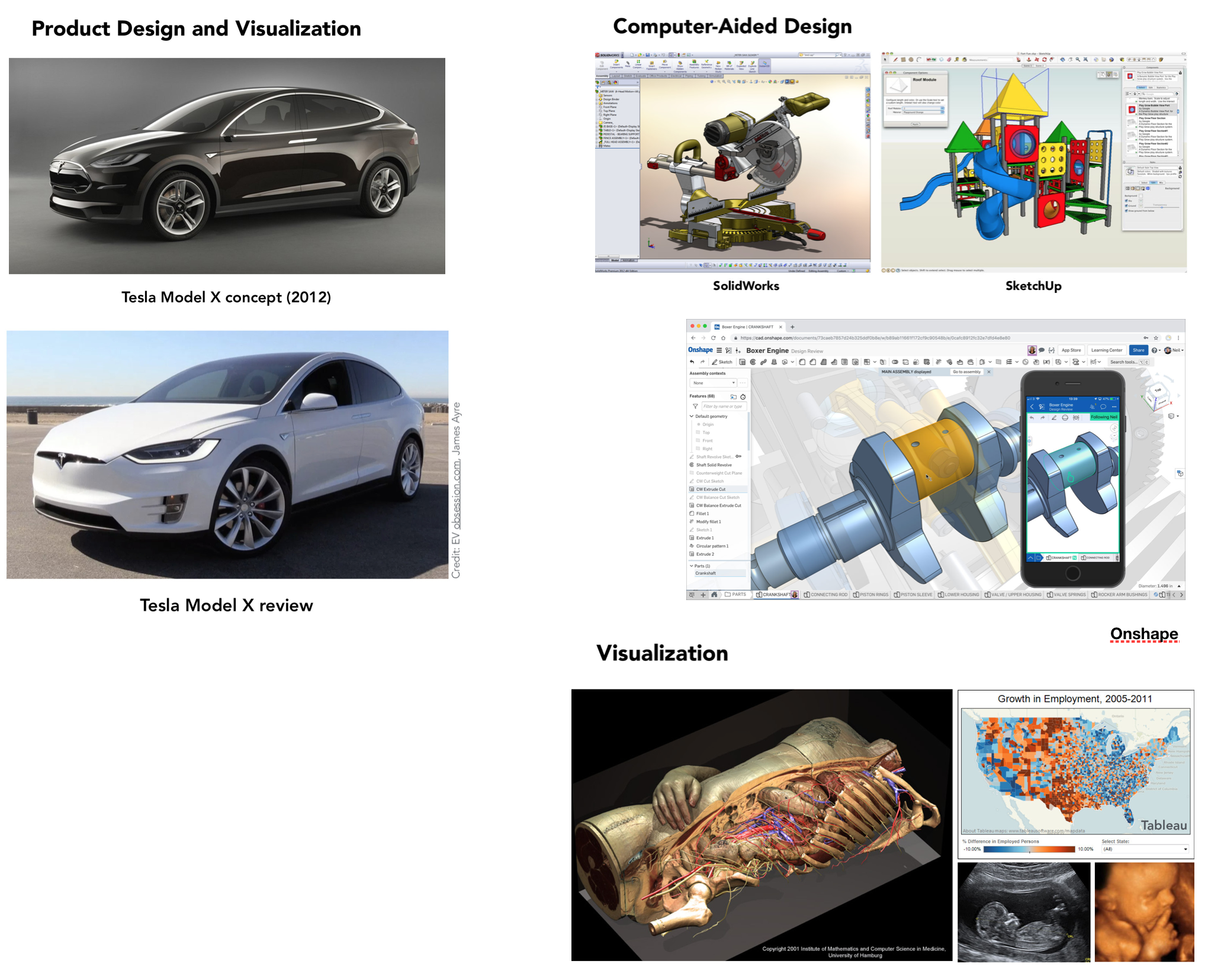
CG is used in the arts: graphical user interfaces, digital photography, graphic design, and fine arts.
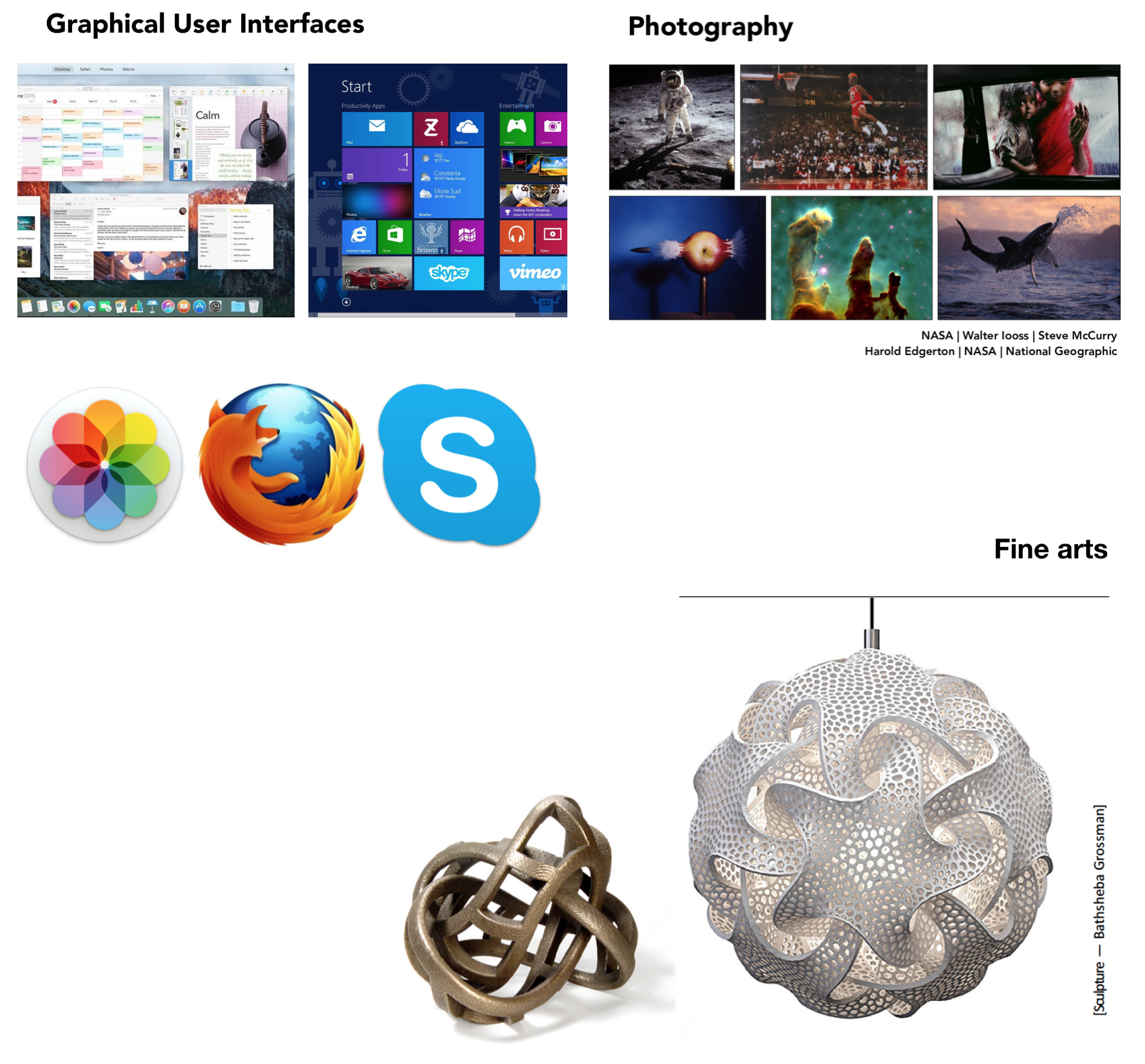
Remarkably, all of the applications we see here are based, at their core, on linear algebra.
Today we’ll start to unlock the methods of computer graphics and see how they depend on linear algebra.
To do that, we’ll go back to the notion of a linear transformation.
Linear Transformations
In the lecture on linear transformations and matrices we talked about linear transformations of \(\mathbb{R}^2\):
- Reflection
- over the \(x_1\) or \(x_2\) axes,
- over the lines \(x_2=x_1\) or \(x_2=-x_1\), and
- through the origin.
- Horizontal and vertical dilation and contraction.
- Horizontal and vertical shearing.
- Projection onto the \(x_1\) or \(x_2\) axes or onto a line through the origin.
Today, we’ll talk about 3D transformations: linear transformations on \(\mathbb{R}^3\).
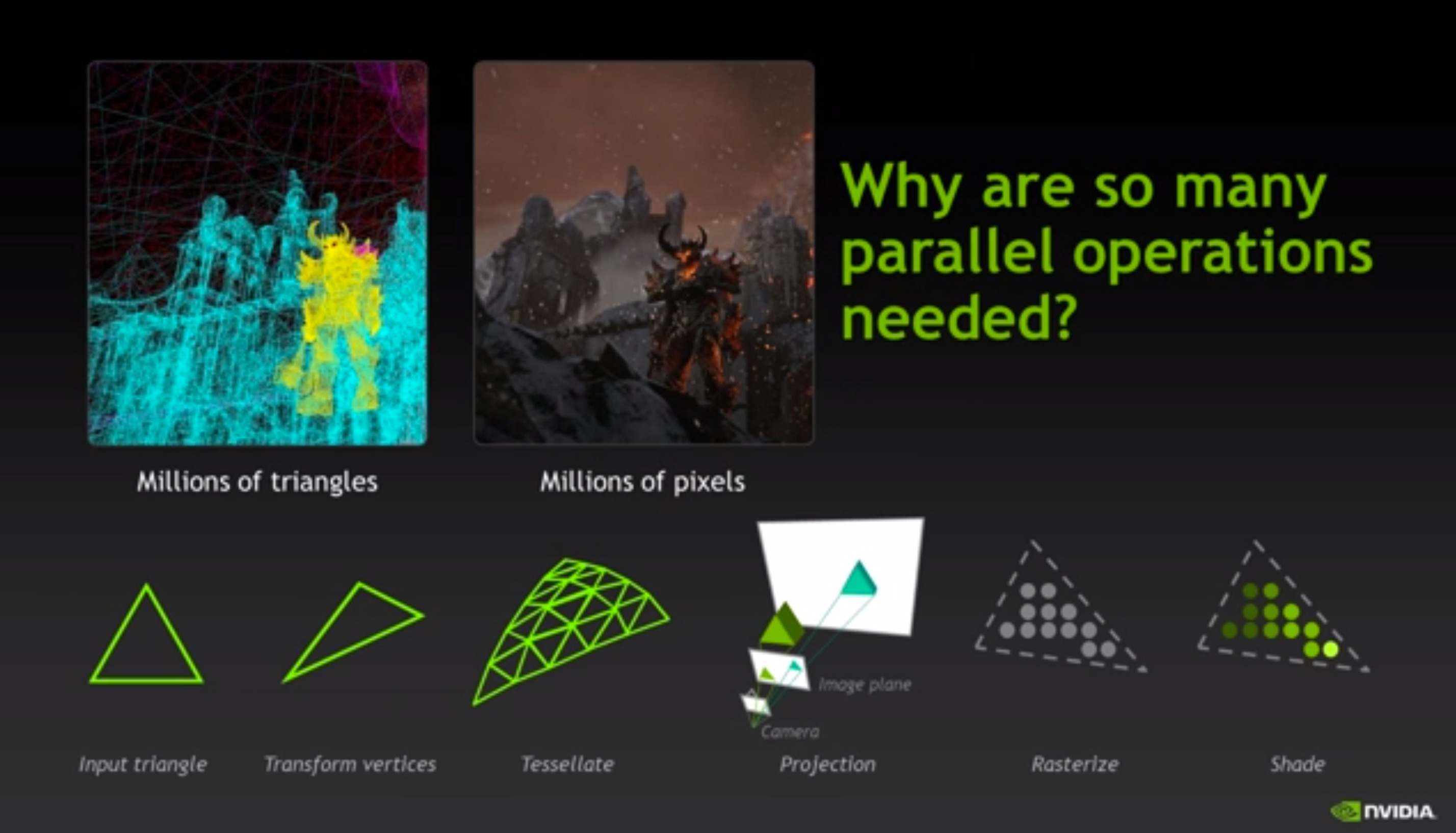
The computer graphics seen in movies and videogames works in three stages:
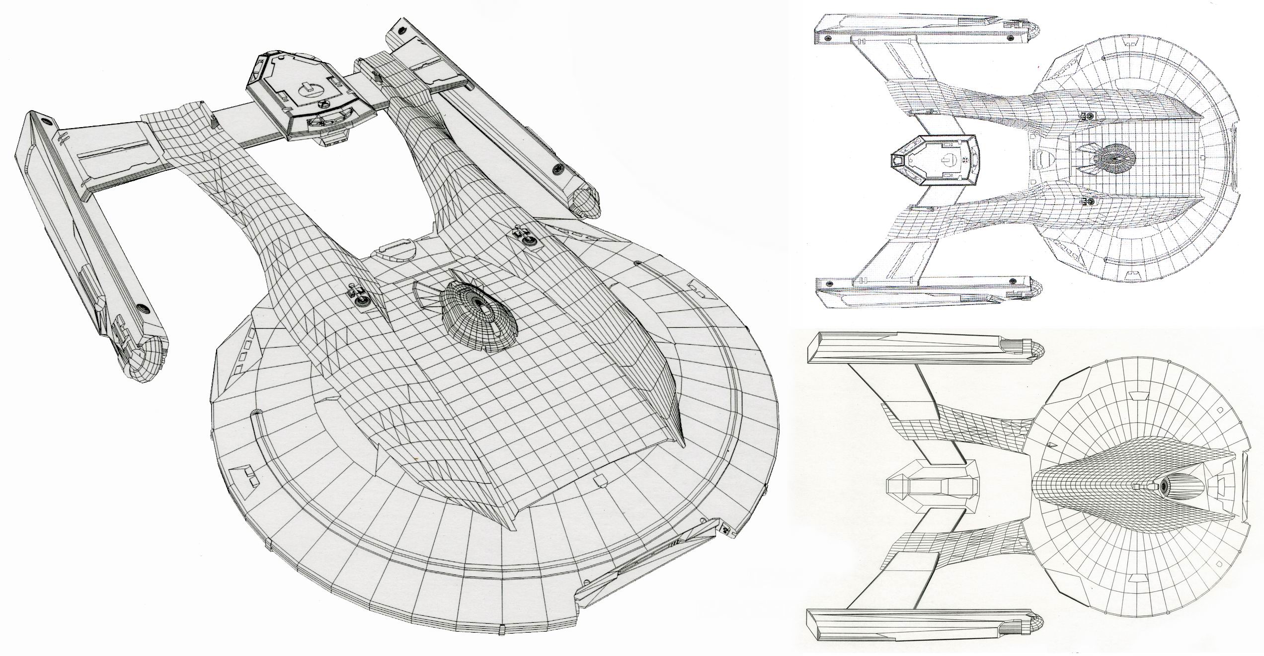
- A 3D model of the scene objects is created;
- The model is converted into (many small) polygons in 3D that approximate the surfaces of the model; and
- The polygons are transformed via a linear transformation to yield a 2D representation that can be shown on a flat screen.
There is interesting mathematics in each stage, but the transformations that take place in the third stage are linear, and that’s what we’ll study today.
Initially, object models may be expressed in terms of smooth functions like polynomials.
However the first step is to convert those smooth functions into a set of discrete pieces – coordinates and line segments.
All subsequent processing is done in terms of the discrete coordinates that approximate the shape of the original model.
The reason for this conversion is that most transformations needed in graphics are linear.
Expressing the scene in terms of coordinates is equivalent to expressing it in terms of vectors, that is, in \(\mathbb{R}^3\).
And linear transformations on vectors are always matrix multiplications, so implementation is simple and uniform.
The resulting representation consists of lists of 3D coordinates called faces. Each face is a polygon.
The lines drawn between coordinates are implied by the way that coordinates are grouped into faces.
The Coordinate System
The standard coordinate system used in computer graphics places the axes in this relationship:
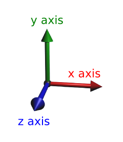
Note the relative position of three axes. We generally think of the \(z\)-axis as coming out of the screen towards us.
We consider the columns of the identity – \(\mathbf{e}_1, \mathbf{e}_2,\) and \(\mathbf{e}_3\) – to be associated with the \(x\), \(y\), and \(z\) directions in this figure.
An Example
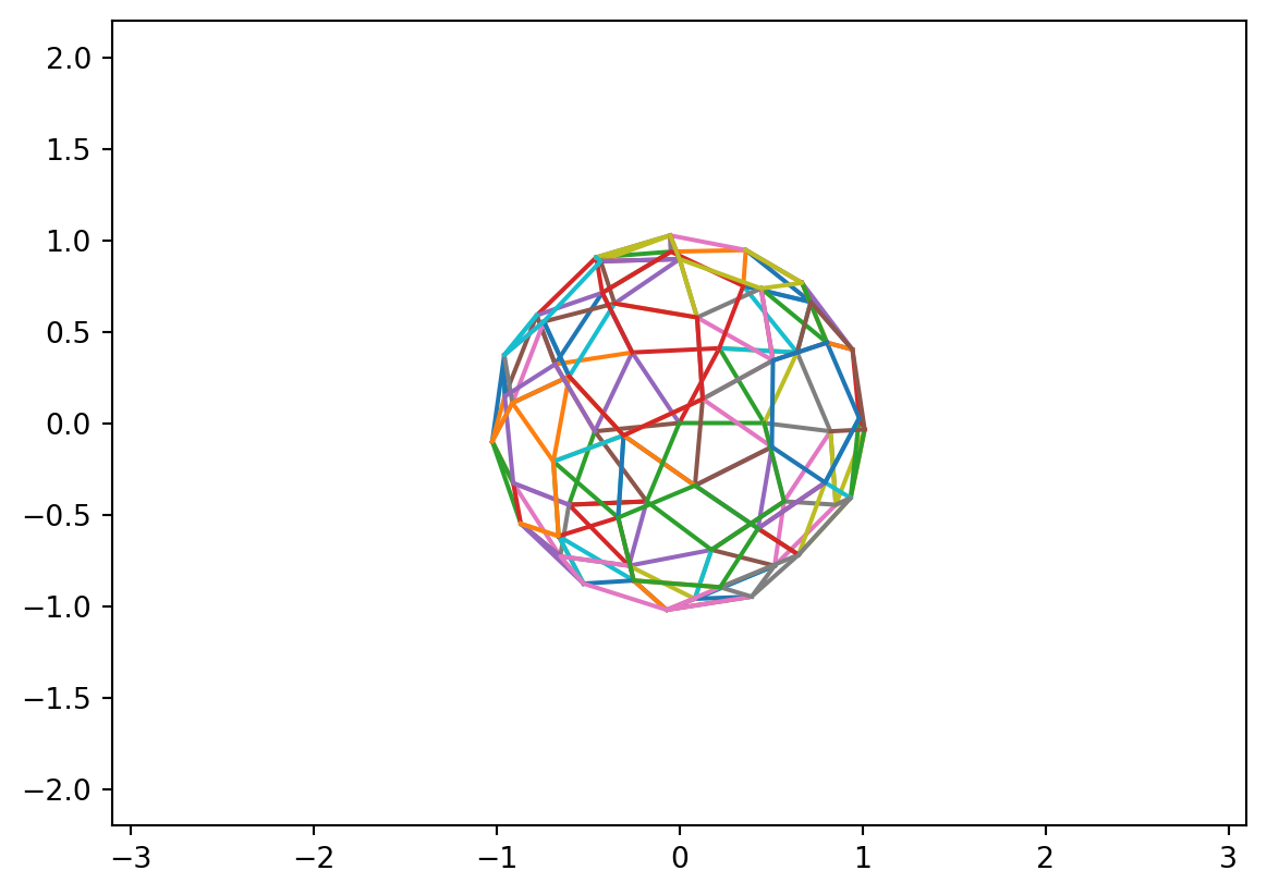
Here is a view of a ball-like object. It is centered at the origin.
The ball is represented in terms of 3D coordinates, but we are only plotting the \(x\) and \(y\) coordinates here.
Colors correspond to faces.
Rotation
Imagine that we want to circle the camera around the ball by moving sideways. In terms of what we would see through the camera, this is equivalent to rotating the ball around the \(y\) axis.
Rotation is a linear transformation. We can implement it by multiplying the coordinates of the ball by a rotation matrix. To define the rotation matrix, we need to think about what happens to each of the columns of \(I: \mathbf{e}_1, \mathbf{e}_2,\) and \(\mathbf{e}_3.\)
To rotate through an angle of \(\alpha\) radians around the \(y\) axis,
the vector \({\bf e_1} = \left[\begin{array}{r}1\\0\\0\end{array}\right]\) goes to \(\left[\begin{array}{c}\cos \alpha\\0\\-\sin \alpha\end{array}\right].\)
Of course, \({\bf e_2}\) is unchanged.
And \({\bf e_3} = \left[\begin{array}{r}0\\0\\1\end{array}\right]\) goes to \(\left[\begin{array}{c}\sin \alpha\\0\\\cos \alpha\end{array}\right].\)
So the entire rotation matrix is:
\[\begin{bmatrix}\cos \alpha&0&\sin \alpha\\0&1&0\\-\sin \alpha&0&\cos\alpha\end{bmatrix}.\]
Translation
Manipulating graphics objects using matrix multiplication is very convenient.
However, there is a commonly used operation that is not a linear transformation: translation – that is, movement in space.
Remember that a transformation \(T(x)\) is linear if \(T(x + y) = T(x) + T(y)\) and \(T(cx) = cT(x)\).
Now, if \(T(x)\) is a translation, then \(T(x) = x + b\) for some nonzero \(b\).
But then \(T(x + y) \neq T(x) + T(y)\).
So a translation is not a linear transformation.
There is a nice way to avoid this difficulty, while keeping things linear.
We will use what are called homogeneous coordinates.
When using homogeneous coordinates, we add another component to the vector representing a point.
The coordinates of the point in \(\mathbb{R}^4\) are the homogeneous coordinates for the point in \(\mathbb{R}^3.\)
The extra component gives us a constant that we can scale and add to the other coordinates, as needed, via matrix multiplication.
This means for 3D graphics, all transformation matrices are \(4\times 4.\)
Example
Let’s say we want to move a point \((x, y, z)\) to location \((x+h, y+k, z+m).\)
We represent the point in homogeneous coordinates as \(\left[\begin{array}{r}x\\y\\z\\1\end{array}\right].\)
The transformation corresponding to this ‘translation’ is:
\[\left[\begin{array}{cccc}1&0&0&h\\0&1&0&k\\0&0&1&m\\0&0&0&1\end{array}\right]\left[\begin{array}{r}x\\y\\z\\1\end{array}\right] = \left[\begin{array}{c}x+h\\y+k\\z+m\\1\end{array}\right].\]
If we only consider \(x, y,\) and \(z\) this is not a linear transformation. But of course, in \(\mathbb{R}^4\) this most definitely is a linear transformation.
We have ‘sheared’ in the fourth dimension, which affects the other three. A very useful trick!
Constructing Matrices for Homogeneous Coordinates
For any transformation \(A\) that is linear in \(\mathbb{R}^3\) (such as scaling, rotation, reflection, shearing, etc.), we can construct the corresponding matrix for homogeneous coordinates quite simply:
If
\[ A = \begin{bmatrix}\blacksquare&\blacksquare&\blacksquare\\\blacksquare&\blacksquare&\blacksquare\\\blacksquare&\blacksquare&\blacksquare\end{bmatrix} \]
Then the corresponding transformation for homogeneous coordinates is:
\[\begin{bmatrix}\blacksquare&\blacksquare&\blacksquare&0\\\blacksquare&\blacksquare&\blacksquare&0\\\blacksquare&\blacksquare&\blacksquare&0\\0&0&0&1\end{bmatrix}\]
In other words, when performing a linear transformation on \(x, y\), and \(z\), one simply ‘carries along’ the extra coordinate without modifying it.
Matrices for 3D Transformations
\[\begin{bmatrix} s_x&0&0&0 \\ 0&s_y&0&0 \\0&0&s_z&0 \\0&0&0&1\end{bmatrix}\]
Translation
\[\begin{bmatrix} 1&0&0&h\\0&1&0&k\\0&0&1&m\\0&0&0&1\end{bmatrix}\]
Rotation around x-, y-, z- axis couterclockwise and looking towards the origin
\[R_x(\alpha)=\begin{bmatrix}1&0&0&0\\ 0&\cos \alpha&-\sin \alpha&0\\0&\sin \alpha&\cos\alpha&0\\0&0&0&1\end{bmatrix}.\]
\[R_y(\alpha)=\begin{bmatrix}\cos \alpha&0&\sin \alpha&0\\0&1&0&0\\-\sin \alpha&0&\cos\alpha&0\\0&0&0&1\end{bmatrix}.\]
\[R_z(\alpha)=\begin{bmatrix}\cos \alpha&-\sin \alpha&0&0\\\sin \alpha&\cos\alpha&0&0\\0&0&1&0\\0&0&0&1\end{bmatrix}.\]
Perspective Projections
There is another nonlinear transformation that is important in computer graphics: perspective.
Happily, we will see that homogeneous coordinates allow us to capture this too as a linear transformation in \(\mathbb{R}^4\).
The eye, or a camera, captures light (essentially) in a single location, and hence gathers light rays that are converging.
So, to portray a scene with realistic appearance, it is necessary to reproduce this effect.
The effect can be thought of as “nearer objects are larger than further objects.”
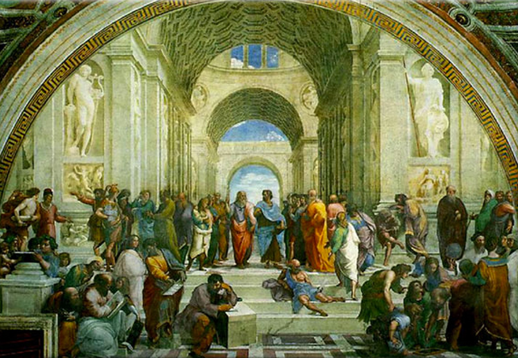
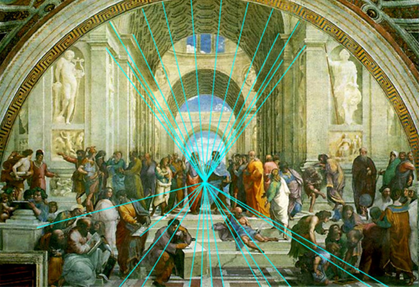
This was (re)discovered by Renaissance artists (supposedly first by Filippo Brunelleschi, around 1405).
Here is a famous example: Raphael’s School of Athens (1510).
Images from here.

My photograph, in the Isabella Stewart Gardner Museum, Boston.
Annunciation by Piermatteo d’Amelia, 1475

My photograph, in the Isabella Stewart Gardner Museum, Boston.
The Tragedy of Lucretia by Sandro Botticelli, 1500
We now understand that this effect interacts in a powerful way with neural circuitry in our brains.
The mind reconstructs a sense of three dimensions from the two dimensional information presented to it by the retina.
This is done by sophisticated processing in the visual cortex, which is a fairly large portion of the brain.
Notice that when the image is stationary, it appears flat (like a picture frame). As soon as it starts to move, it springs into 3D in perception.
Computing Perspective
To render a scene with perspective, we simply have to consider how objects appear when viewed from a point (like an eye or a camera).
Figures from Linear Alegebra and its Applications, Lay, Lay, and MacDonald.
A standard setup for computing a perspective transformation is as shown in this figure:
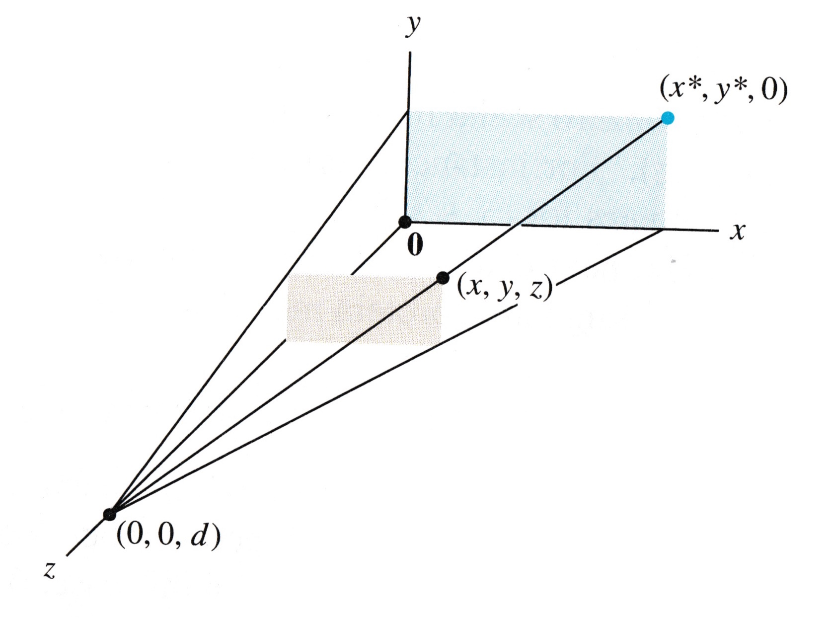
For simplicity, we will let the \(xy\)-plane represent the screen. This is called the viewing plane.
The eye/camera is located on the \(z\) axis, at the point \((0,0,d)\). This is call the center of projection.
A perspective projection maps each point \((x,y,z)\) onto an image point \((x^*,y^*,0)\) so that the center of projection and the two points are all on the same line.
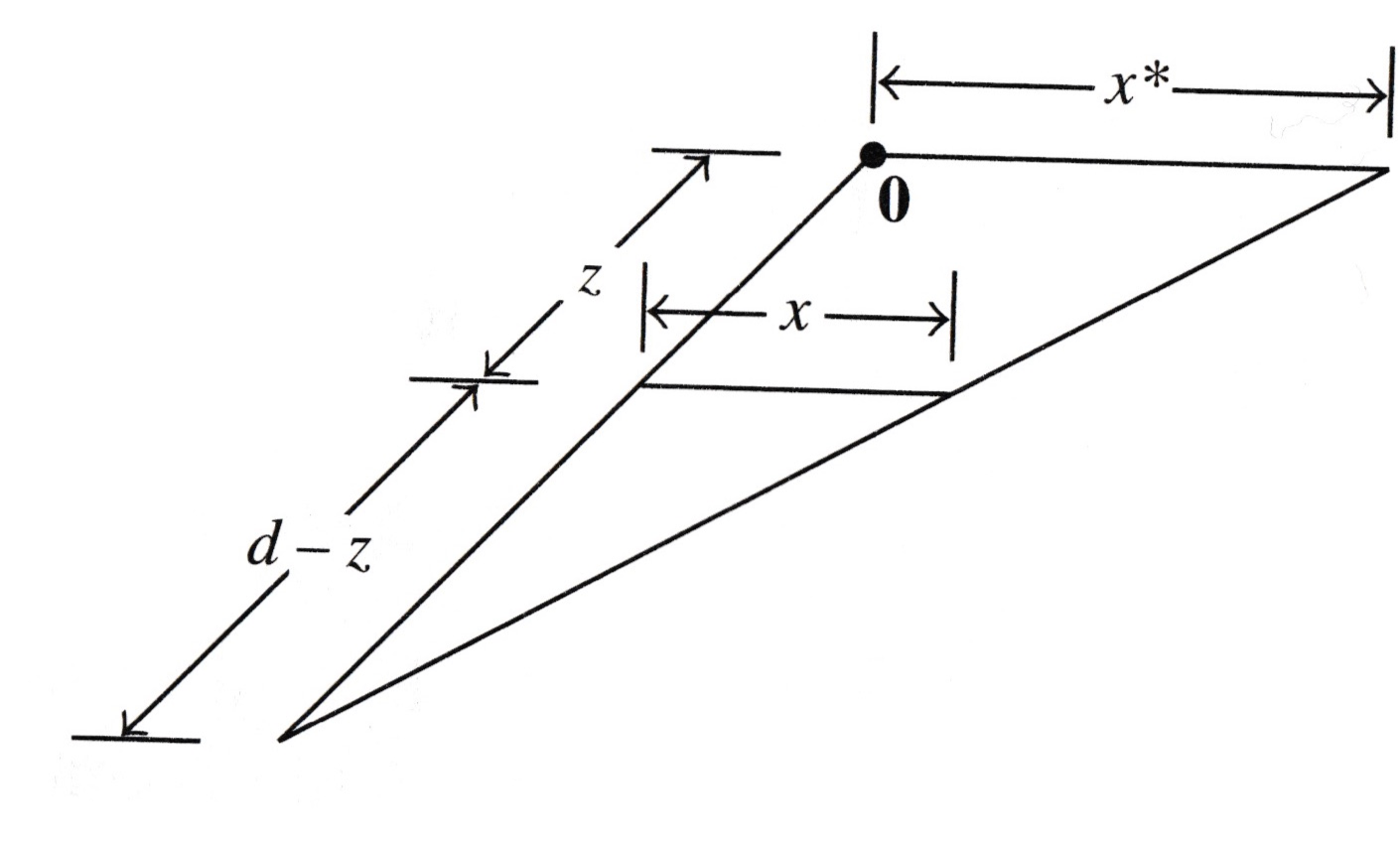
We can compute the projection transformation using similar triangles.
The triangle in the \(xz\)-plane shows the lengths of corresponding line segments.
Similar triangles show that
\[\frac{x^*}{d} = \frac{x}{d-z}\]
and so
\[x^*=\frac{dx}{d-z}\;=\;\frac{x}{1-z/d}.\]
Notice that the function \(T: (x,z)\mapsto\frac{x}{1-z/d}\) is not linear.
However, using homogeneous coordinates, we can construct a linear version of \(T\) in \(\mathbb{R}^4.\)
To do so, we establish the following convention: we will allow the fourth coordinate to vary away from 1.
However, when we plot, for a point \(\begin{bmatrix}x\\y\\z\\\end{bmatrix}\) we will plot the point \(\begin{bmatrix}\frac{x}{h}\\\frac{y}{h}\\\frac{z}{h}\end{bmatrix}.\)
In this way, by dividing the \(x,y,z\) coordinates by the \(h\) coordinate, we can implement a nonlinear transform in \(\mathbb{R}^3.\)
So, to implement the perspective transform, we want \(\begin{bmatrix}x\\y\\z\\1\end{bmatrix}\) to map to \(\begin{bmatrix}\frac{x}{1-z/d}\\\frac{y}{1-z/d}\\0\\1\end{bmatrix}.\)
The way we will implement this is to actually cause it to map to \(\begin{bmatrix}x\\y\\0\\1-z/d\end{bmatrix}.\)
Then, when we plot (dividing \(x\) and \(y\) by the \(h\) value) we will get the proper transform.
The matrix that implements this transformation is quite simple:
\[\begin{bmatrix}1&0&0&0\\0&1&0&0\\0&0&0&0\\0&0&-1/d&1\end{bmatrix}.\]
So:
\[\begin{bmatrix}1&0&0&0\\0&1&0&0\\0&0&0&0\\0&0&-1/d&1\end{bmatrix}\begin{bmatrix}x\\y\\z\\1\end{bmatrix} = \begin{bmatrix}x\\y\\0\\1-z/d\end{bmatrix}.\]
Composing Transformations
One big payoff for casting all graphics operations as linear transformations comes in the composition of transformations.
Consider two linear transformations \(T\) and \(S\). For example, \(T\) could be a scaling and \(S\) could be a rotation. Assume \(S\) is implemented by a matrix \(A\) and \(T\) is implemented by a matrix \(B\).
To first scale and then rotate a vector \(\mathbf{x}\) we would compute \(S(T(\mathbf{x}))\).
Of course this is implemented as \(A(B\mathbf{x}).\)
But note that this is the same as \((AB)\mathbf{x}.\) In other words, \(AB\) is a single matrix that both scales and rotates \(\mathbf{x}\).
By extension, we can combine any arbitrary sequence of linear transformations into a single matrix. This greatly simplifies high-speed graphics.
Note though that if \(C = AB\), then \(C\) is the transformation that first applies \(B\), then applies \(A\) (order matters).
Example. Let’s work in homogenous coordinates for points in \(\mathbb{R}^2\). Find the \(3\times 3\) matrix that corresponds to the composite transformation of first scaling by 0.3, then rotation of 90\(^\circ\) about the origin, and finally a translation of \(\begin{bmatrix}-0.5\\2\end{bmatrix}\) to each point of a figure.
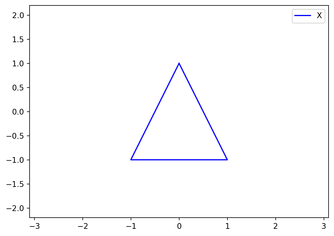
We’ll use this triangle to show the sequence of transformations.
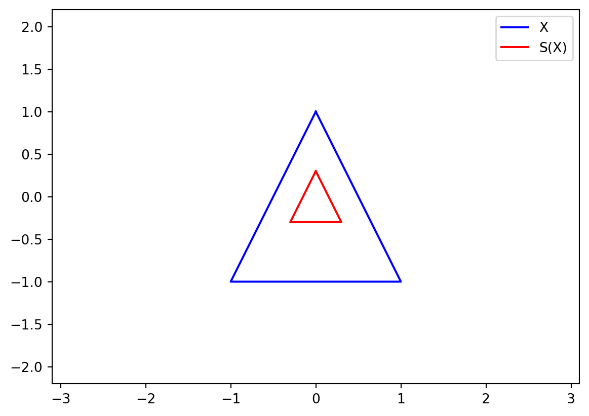
Scaling by 0.3.
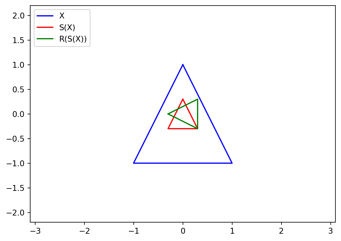
Scaling by 0.3, then rotating by 90\(^\circ\) about the origin.
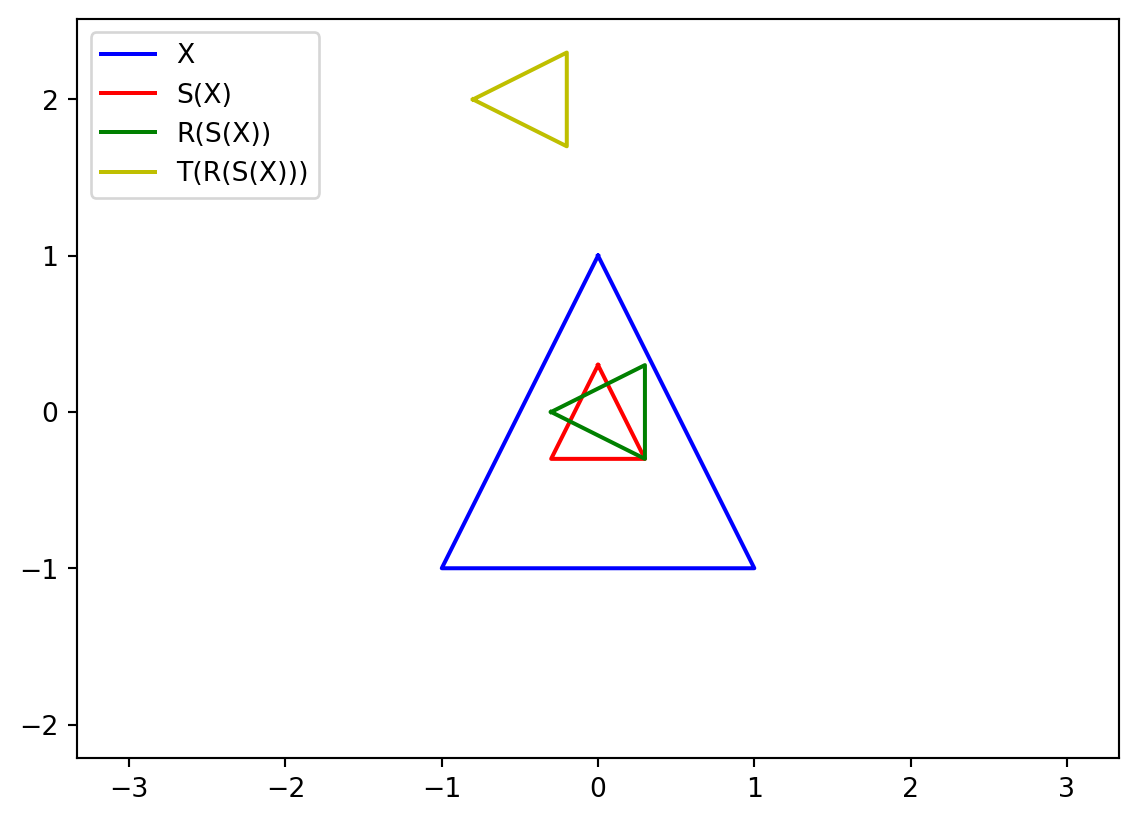
Scaling by 0.3, then rotation of 90\(^\circ\) about the origin, then translation of \(\begin{bmatrix}-0.5\\2\end{bmatrix}\).
Let’s see how to compose these three transformations into a single matrix multiplication.
The scaling matrix is:
\[S = \begin{bmatrix}0.3&0&0\\0&0.3&0\\0&0&1\end{bmatrix}\]
The rotation matrix is:
\[R = \begin{bmatrix}0&-1&0\\1&0&0\\0&0&1\end{bmatrix}\]
(Note that \(\sin 90^\circ = 1\) and \(\cos 90^\circ = 0.\))
The translation matrix is:
\[T = \begin{bmatrix}1&0&-0.5\\0&1&2\\0&0&1\end{bmatrix}\]
So the matrix for the composite transformation is:
\[TRS = \begin{bmatrix}1&0&-0.5\\0&1&2\\0&0&1\end{bmatrix}\begin{bmatrix}0&-1&0\\1&0&0\\0&0&1\end{bmatrix}\begin{bmatrix}0.3&0&0\\0&0.3&0\\0&0&1\end{bmatrix} = \begin{bmatrix}0&-0.3&-0.5\\0.3&0&2\\0&0&1\end{bmatrix}.\]
Note that \(TRS\) first applies S (scaling), then applis R (rotation), and last applies T (translation).
We need to be careful with the order of the matrices!
Consider a vector \(\mathbf{x}\in \mathbb{R}^2\).
Let \(P\) be projection matrix that projects \(\mathbf{x}\) onto the x-axis and \(R\) be a rotation matrix that rotates \(\mathbf{x}\) by 30\(^\circ\) about the origin.
Note that \(PR \ne RP\):
- \(PR\) first rotates the vector and then applies projection, while
- \(RP\) first projects the vector and then applies rotation.
Homework 7
Homework 7 will allow you to explore these ideas by computing various transformation matrices. I will give you some 3D wireframe objects and you will compute the necessary matrices to create a simple animation.
Here is what your finished product will look like:
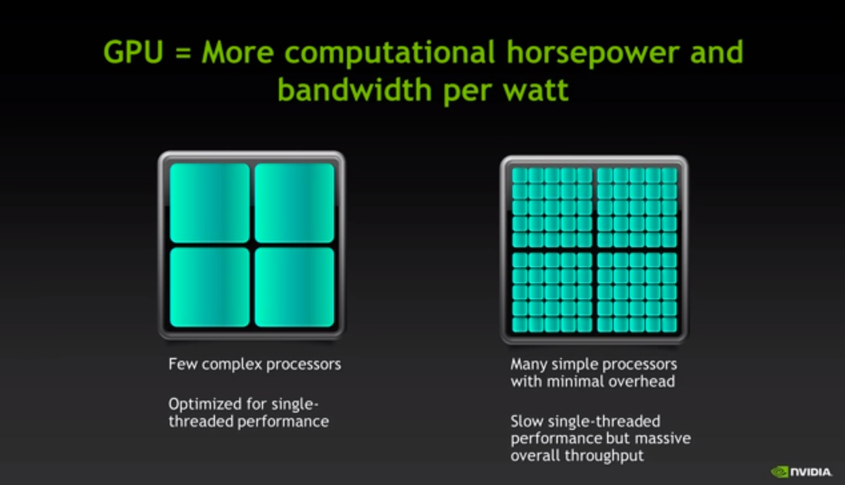
Fast Computation of Linear Systems using Graphics Processing Units (GPUs)
![]()
Examples of Other Linear Systems Used in Computer Graphics
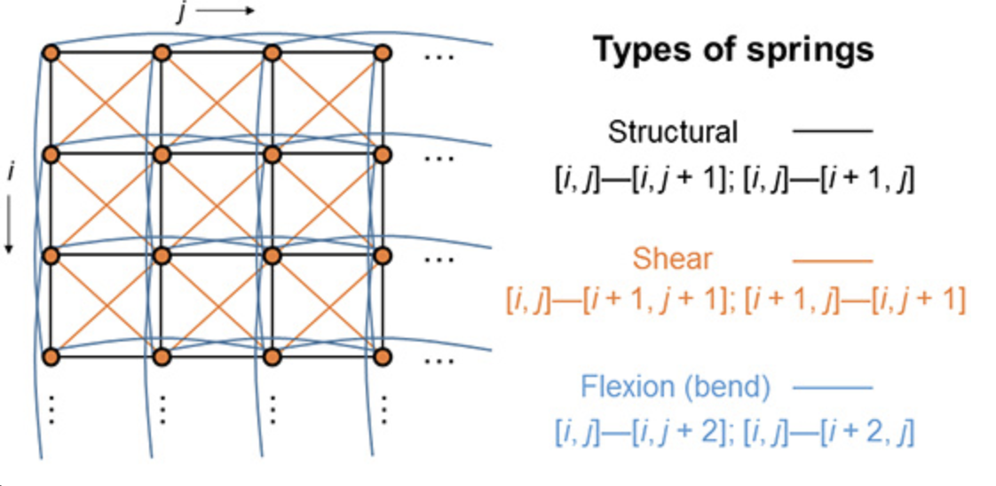
Cloth Simulation
In cloth simulation, we treat the cloth as a collection of particles interconnected with different types of springs. The springs cause the cloth to behave properly with respect to bending, shearing, etc.
Hooke’s Law and Newton’s 2nd Law are used as the equations of motion to capture the cloth behaviors. These are linear difference equations.
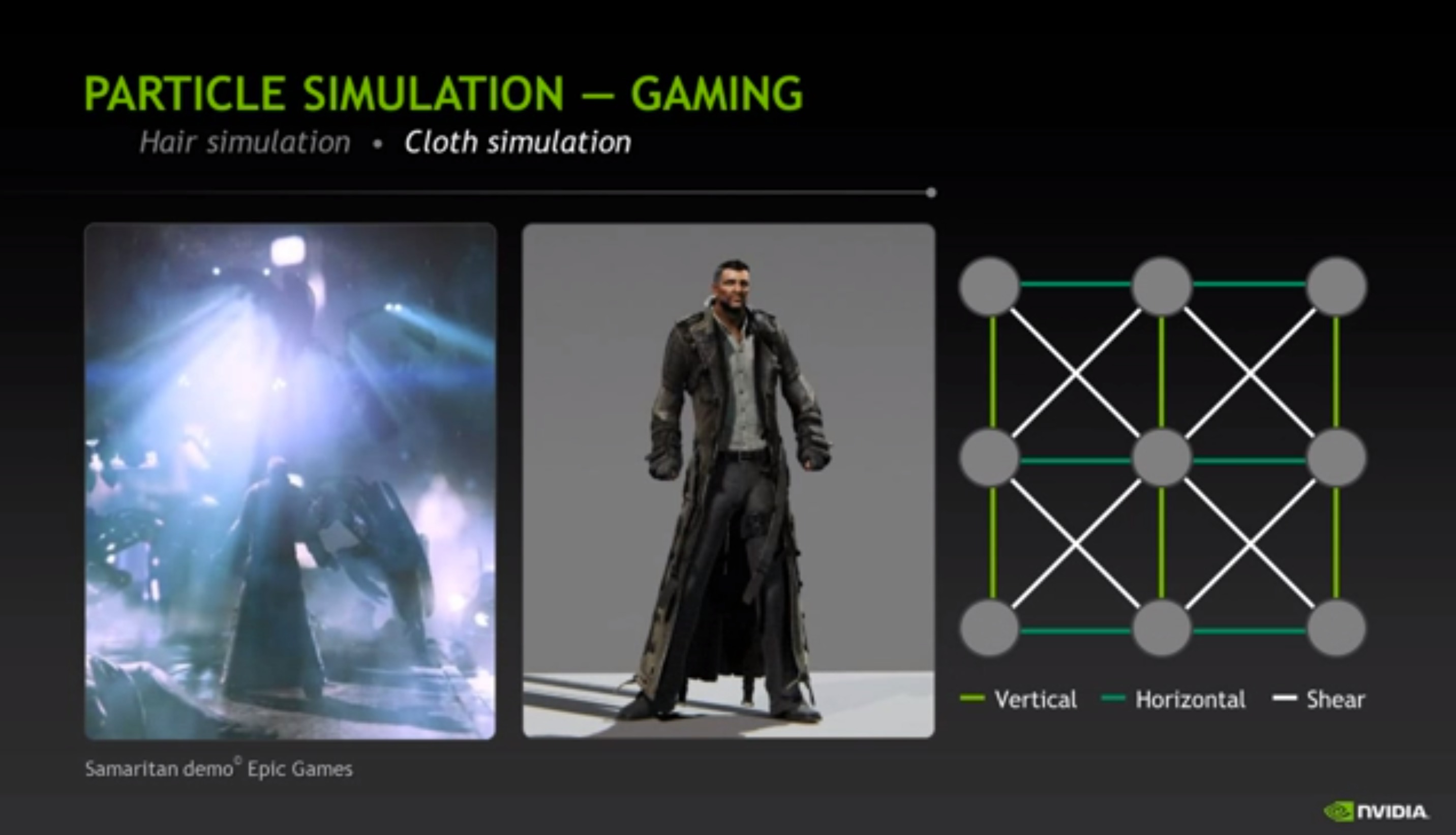
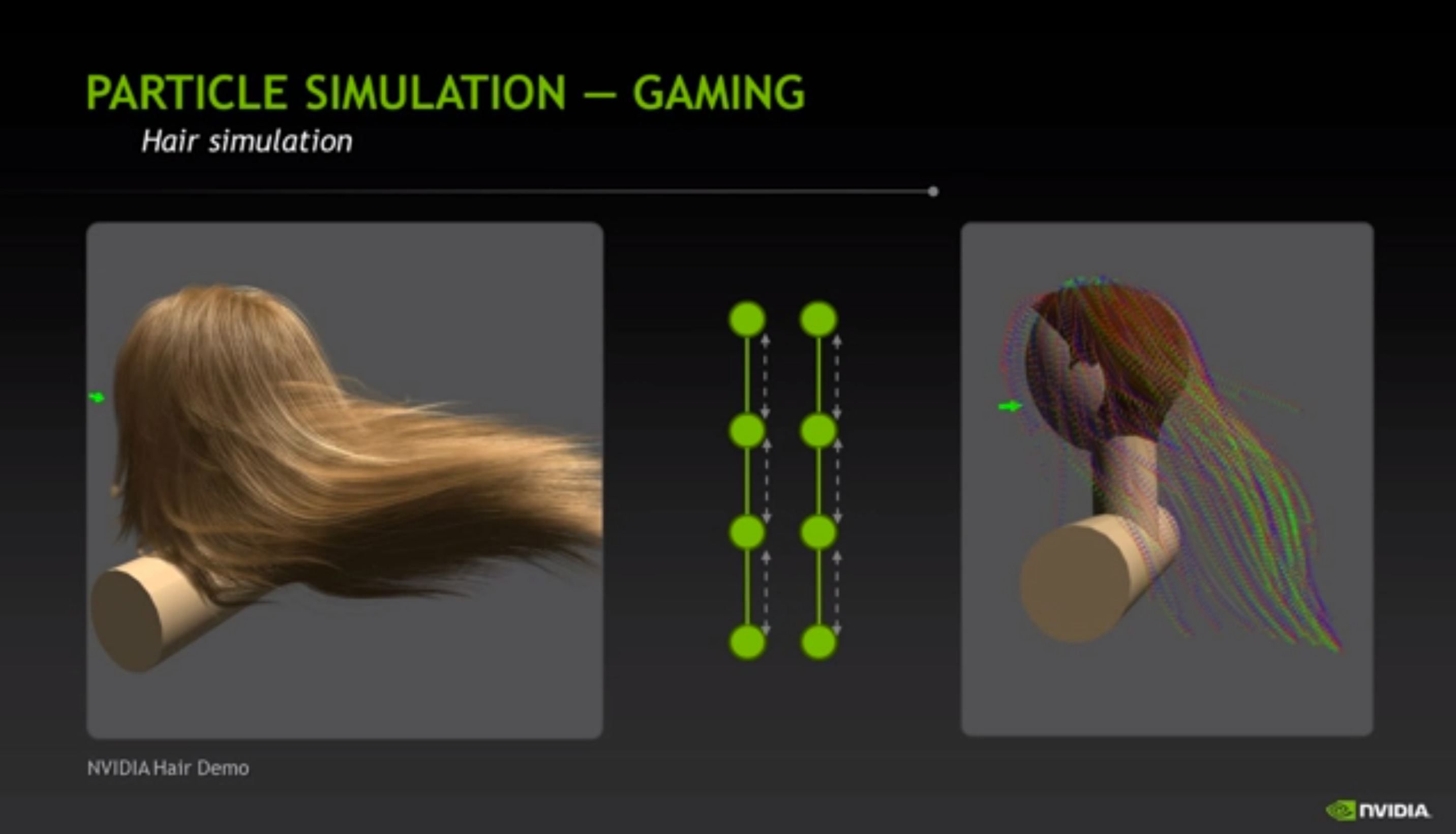
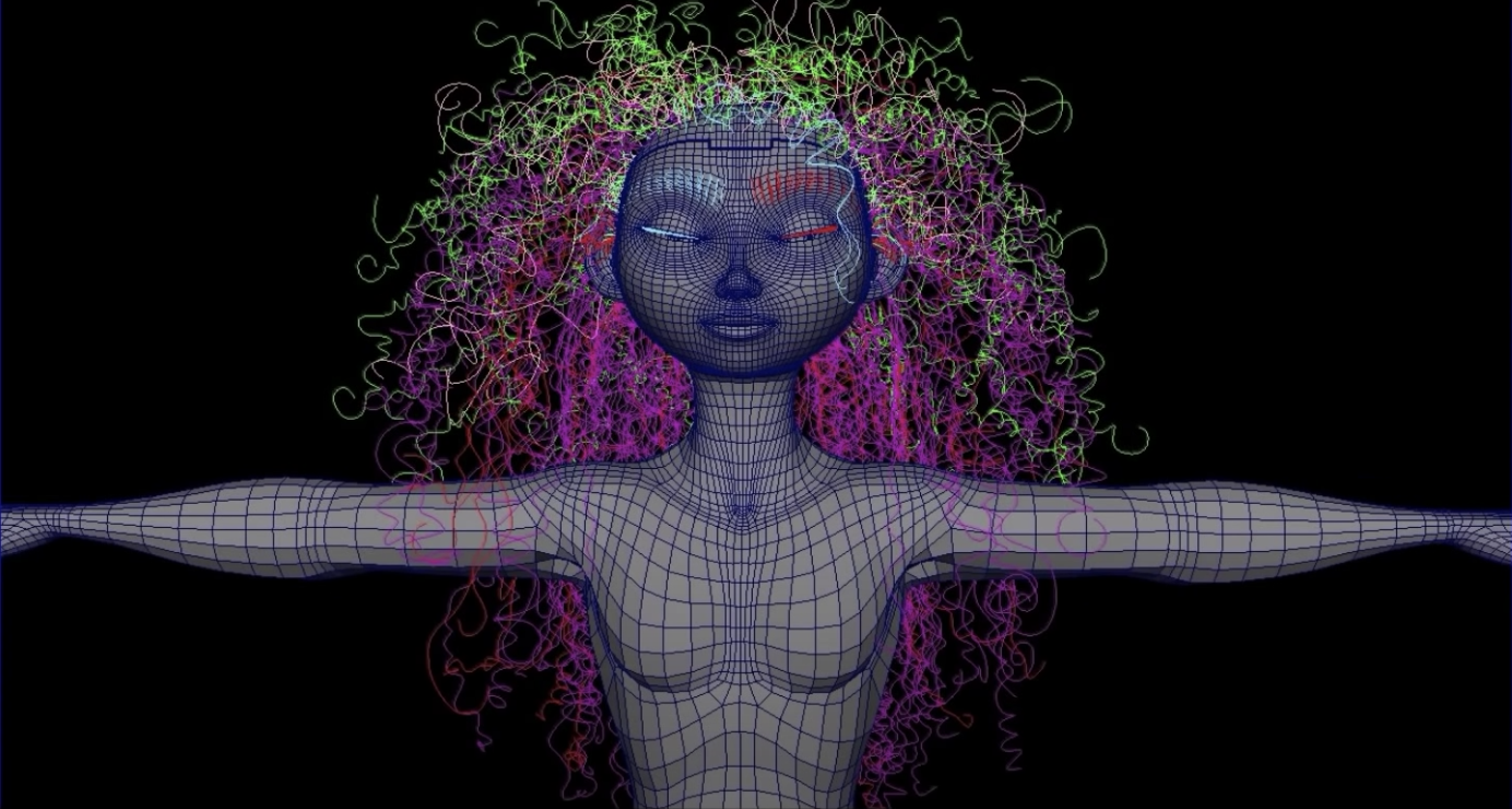
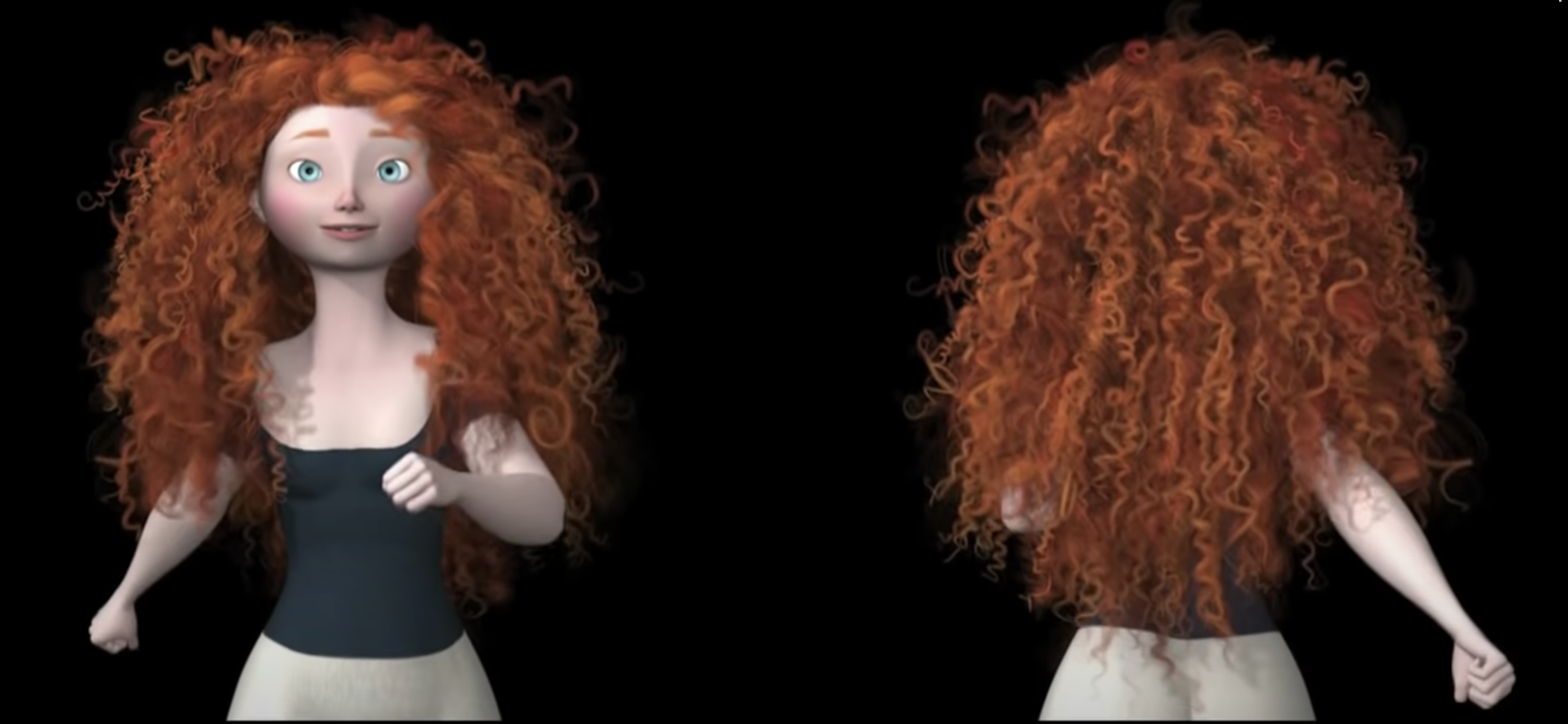
Hair Simulation
A similar strategy is used for hair, except that the connections are 1-D (along each hair strand) instead of 2-D.
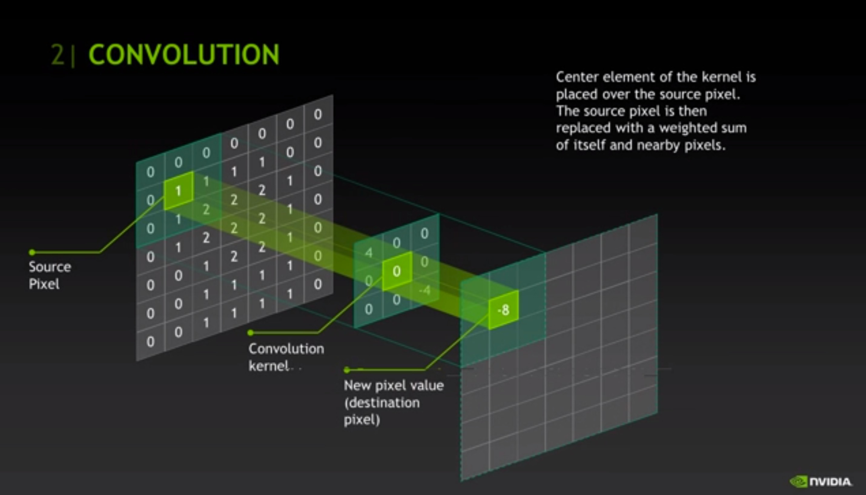
Convolution
Interestingly, the fact that GPUs are optimized for fast convolution was crucial in their adoption for fast machine learning.