[[0 1 1 0]
 [1 1 0 0]]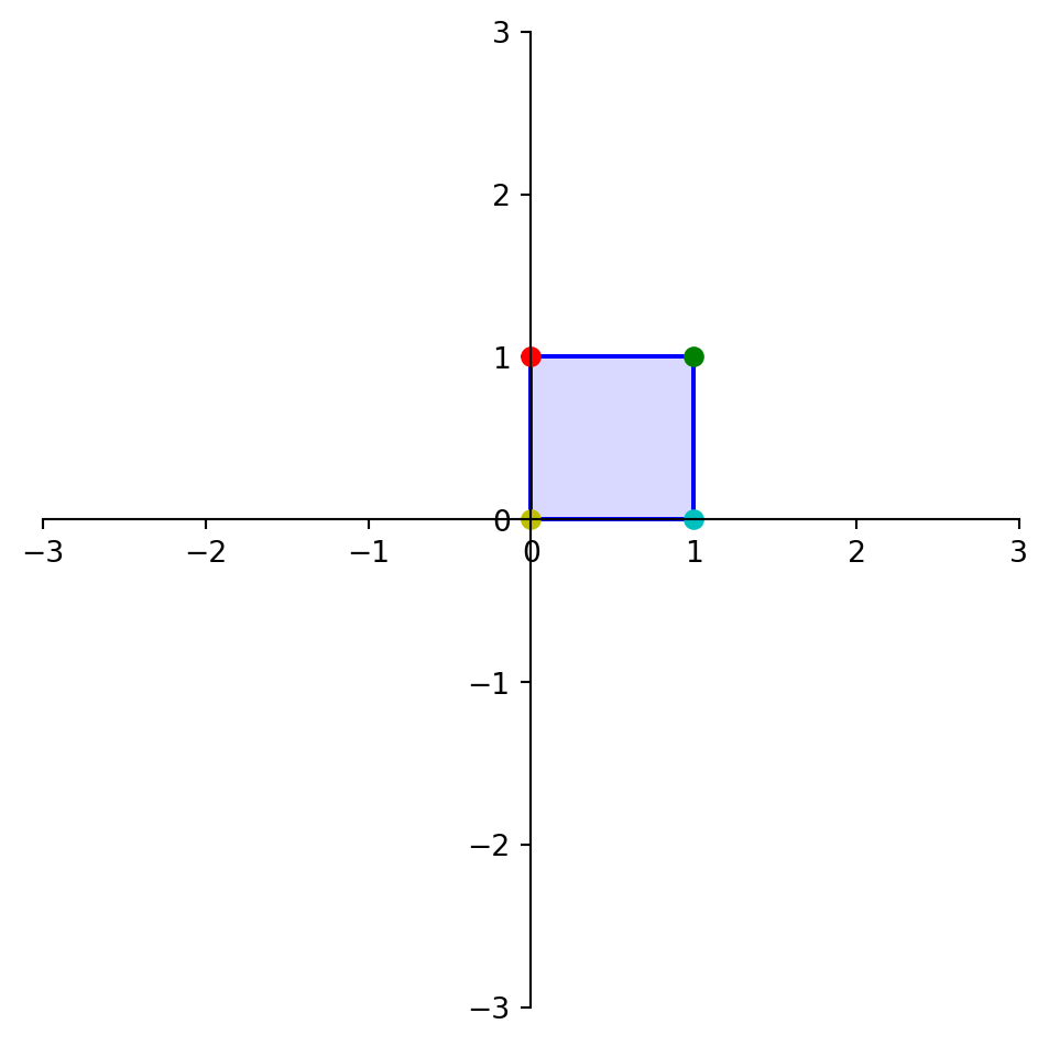
Many parts of this page are based on Linear Algebra and its Applications, by David C. Lay
So far we’ve been treating the matrix equation
\[ A{\bf x} = {\bf b}\]
as simply another way of writing the vector equation
\[ x_1{\bf a_1} + \dots + x_n{\bf a_n} = {\bf b}.\]
However, we’ll now think of the matrix equation in a new way:
We will think of \(A\) as “acting on” the vector \({\bf x}\) to create a new vector \({\bf b}\).
For example, let’s let \(A = \left[\begin{array}{rrr}2&1&1\\3&1&-1\end{array}\right].\) Then we find:
\[ A \left[\begin{array}{r}1\\-4\\-3\end{array}\right] = \left[\begin{array}{r}-5\\2\end{array}\right] \]
In other words, if \({\bf x} = \left[\begin{array}{r}1\\-4\\-3\end{array}\right]\) and \({\bf b} = \left[\begin{array}{r}-5\\2\end{array}\right]\), then \(A\) transforms \({\bf x}\) into \({\bf b}\).
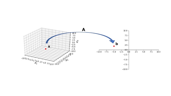
Notice what \(A\) has done: it took a vector in \(\mathbb{R}^3\) and transformed it into a vector in \(\mathbb{R}^2\).
How does this fact relate to the shape of \(A\)?
\(A\) is \(2 \times 3\) — that is, \(A \in \mathbb{R}^{2\times 3}\).
This gives a new way of thinking about solving \(A{\bf x} = {\bf b}\).
To solve \(A{\bf x} = {\bf b}\), we must “search for” the vector(s) \({\bf x}\) in \(\mathbb{R}^3\) that are transformed into \({\bf b}\) in \(\mathbb{R}^2\) under the “action” of \(A\).
For a different \(A\), the mapping might be from \(\mathbb{R}^1\) to \(\mathbb{R}^3\):
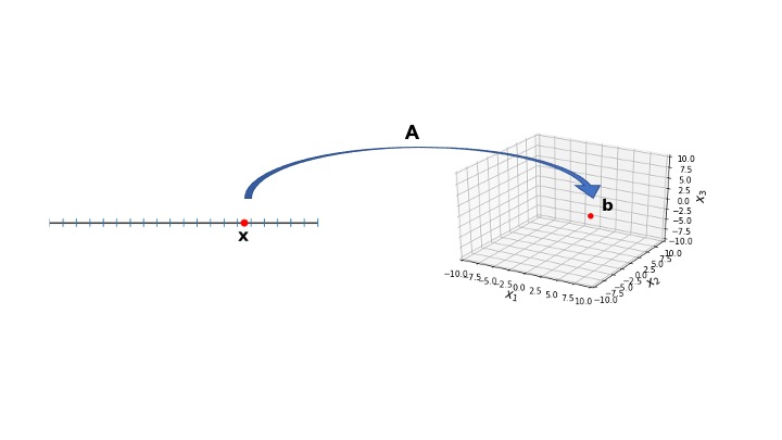
What would the shape of \(A\) be in the above case?
Since \(A\) maps from \(\mathbb{R}^1\) to \(\mathbb{R}^3\), \(A \in \mathbb{R}^{3\times 1}\).
That is, \(A\) has 3 rows and 1 column.
In another case, \(A\) could be a square \(2\times 2\) matrix.
Then, it would map from \(\mathbb{R}^2\) to \(\mathbb{R}^2\):

We have moved out of the familiar world of functions of one variable: we are now thinking about functions that transform a vector into a vector.
Or, put another way, functions that transform multiple variables into multiple variables.
Some terminology:
A transformation (or function or mapping) \(T\) from \(\mathbb{R}^n\) to \(\mathbb{R}^m\) is a rule that assigns to each vector \({\bf x}\) in \(\mathbb{R}^n\) a vector \(T({\bf x})\) in \(\mathbb{R}^m\).
The set \(\mathbb{R}^n\) is called the domain of \(T\), and \(\mathbb{R}^m\) is called the codomain of \(T\).
The notation:
\[ T: \mathbb{R}^n \rightarrow \mathbb{R}^m\]
indicates that the domain of \(T\) is \(\mathbb{R}^n\) and the codomain is \(\mathbb{R}^m\).
For \(\bf x\) in \(\mathbb{R}^n,\) the vector \(T({\bf x})\) is called the image of \(\bf x\) (under \(T\)).
The set of all images \(T({\bf x})\) is called the range of \(T\).

Here, the green plane is the set of all points that are possible outputs of \(T\) for some input \(\mathbf{x}\).
So in this example:
Let’s do an example. Let’s say I have these points in \(\mathbb{R}^2\):
\[ \left[\begin{array}{r}0\\1\end{array}\right],\left[\begin{array}{r}1\\1\end{array}\right],\left[\begin{array}{r}1\\0\end{array}\right],\left[\begin{array}{r}0\\0\end{array}\right]\]
Where are these points located?
[[0 1 1 0]
[1 1 0 0]]
Now let’s transform each of these points according to the following rule. Let
\[ A = \left[\begin{array}{rr}1&1.5\\0&1\end{array}\right]. \]
We define \(T({\bf x}) = A{\bf x}\). Then we have
\[ T: \mathbb{R}^2 \rightarrow \mathbb{R}^2.\]
What is the image of each of these points under \(T\)?
\[ A\left[\begin{array}{r}0\\1\end{array}\right] = \left[\begin{array}{r}1.5\\1\end{array}\right]\]
\[ A\left[\begin{array}{r}1\\1\end{array}\right] = \left[\begin{array}{r}2.5\\1\end{array}\right]\]
\[ A\left[\begin{array}{r}1\\0\end{array}\right] = \left[\begin{array}{r}1\\0\end{array}\right]\]
\[ A\left[\begin{array}{r}0\\0\end{array}\right] = \left[\begin{array}{r}0\\0\end{array}\right]\]
square =
[[0 1 1 0]
 [1 1 0 0]]
A matrix =
[[1.  1.5]
 [0.  1. ]]
transformed square =
[[1.5 2.5 1.  0. ]
 [1.  1.  0.  0. ]]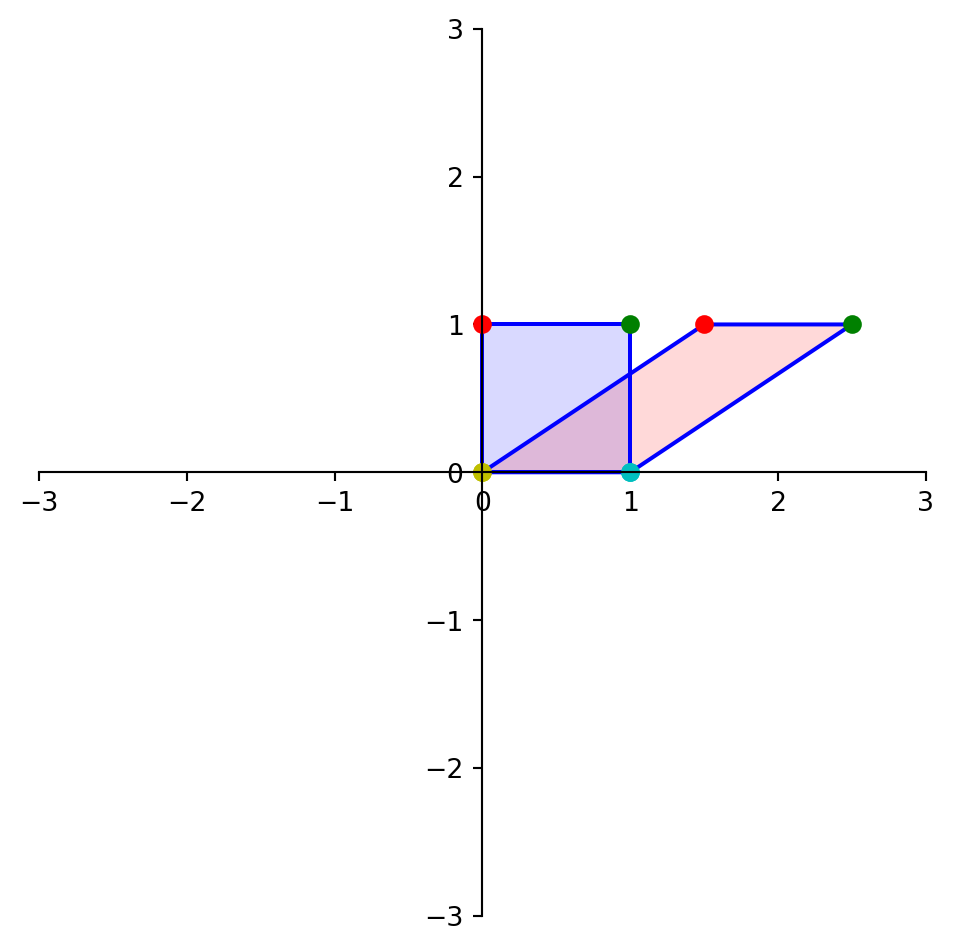
This sort of transformation, where points are successively slid sideways, is called a shear transformation.
By the properties of matrix-vector multiplication, we know that the transformation \({\bf x} \mapsto A{\bf x}\) has the properties that
\[ A({\bf u} + {\bf v}) = A{\bf u} + A{\bf v} \;\;\;\text{and}\;\;\; A(c{\bf u}) = cA{\bf u}\]
for all \(\bf u, v\) in \(\mathbb{R}^n\) and all scalars \(c\).
We are now ready to define one of the most fundamental concepts in the course: the concept of a linear transformation.
(You are now finding out why the subject is called linear algebra!)
Definition. A transformation \(T\) is linear if:
To fully grasp the significance of what a linear transformation is, don’t think of just matrix-vector multiplication. Think of \(T\) as a function in more general terms.
The definition above captures a lot of transformations that are not matrix-vector multiplication. For example, think of:
\[ T(f) = \int_0^1 f(t) \,dt \]
Is \(T\) a linear transformation?
Checking the conditions of our definition:
\[ T(f + g) = T(f) + T(g) \]
in other words:
\[ \int_0^1 f(t) + g(t) \,dt = \int_0^1 f(t) \,dt + \int_0^1 g(t) \,dt\]
and also:
\[ T(c \cdot f) = c \cdot T(f) \]
(check that yourself)
What about:
\[ T(f) = \frac{d f(t)}{dt} \]
Is \(T\) a linear transformation?
What about:
\[ T(x) = e^x \]
Is \(T\) a linear transformation?
A key aspect of a linear transformation is that it preserves the operations of vector addition and scalar multiplication.
For example: for vectors \(\mathbf{u}\) and \(\mathbf{v}\), one can either:
One gets the same result either way. The transformation does not affect the addition.
This leads to two important facts.
If \(T\) is a linear transformation, then
\[ T({\mathbf 0}) = {\mathbf 0} \]
and
\[ T(c\mathbf{u} + d\mathbf{v}) = cT(\mathbf{u}) + dT(\mathbf{v}) \]
In fact, if a transformation satisfies the second equation for all \(\mathbf{u}, \mathbf{v}\) and \(c, d,\) then it must be a linear transformation.
Both of the rules defining a linear transformation derive from this single equation.
Example.
Given a scalar \(r\), define \(T: \mathbb{R}^2 \rightarrow \mathbb{R}^2\) by \(T(\mathbf{x}) = r\mathbf{x}\).
(\(T\) is called a contraction when \(0\leq r \leq 1\) and a dilation when \(r > 1\).)
Let \(r = 3\), and show that \(T\) is a linear transformation.
Solution.
Let \(\mathbf{u}, \mathbf{v}\) be in \(\mathbb{R}^2\) and let \(c, d\) be scalars. Then
\[ T(c\mathbf{u} + d\mathbf{v}) = 3(c\mathbf{u} + d\mathbf{v}) \]
\[ = 3c\mathbf{u} + 3d\mathbf{v} \]
\[ = c(3\mathbf{u}) + d(3\mathbf{v}) \]
\[ = cT(\mathbf{u}) + dT(\mathbf{v}) \]
Thus \(T\) is a linear transformation because it satisfies the rule \(T(c\mathbf{u} + d\mathbf{v}) = cT(\mathbf{u}) + dT(\mathbf{v})\).
Example.
Let \(T(\mathbf{x}) = \mathbf{x} + \mathbf{b}\) for some \(\mathbf{b} \neq 0\).
What sort of operation does \(T\) implement?
Answer: translation.
Is \(T\) a linear transformation?
Solution.
We only need to compare
\[T(\mathbf{u} + \mathbf{v})\]
to
\[T(\mathbf{u}) + T(\mathbf{v}).\]
So:
\[T(\mathbf{u} + \mathbf{v}) = \mathbf{u} + \mathbf{v} + \mathbf{b}\]
and
\[T(\mathbf{u}) + T(\mathbf{v}) = (\mathbf{u} + \mathbf{b}) + (\mathbf{v} + \mathbf{b})\]
If \(\mathbf{b} \neq 0\), then the above two expressions are not equal.
So \(T\) is not a linear transformation.
A company manufactures two products, B and C. To do so, it requires materials, labor, and overhead.
For one dollar’s worth of product B, it spends 45 cents on materials, 25 cents on labor, and 15 cents on overhead.
For one dollar’s worth of product C, it spends 40 cents on materials, 30 cents on labor, and 15 cents on overhead.
Let us construct a “unit cost” matrix:
\[U = \begin{array}{r} \begin{array}{rrr}\text{B}&\;\;\;\;\text{C}\;&\;\;\;\;\;\;\;\;\;\;\;\end{array}\\ \left[\begin{array}{rr}.45&.40\\.25&.30\\.15&.15\end{array}\right] \begin{array}{r}\text{Materials}\\\text{Labor}\\\text{Overhead}\end{array}\\ \end{array}\]
Let \(\mathbf{x} = \left[\begin{array}{r}x_1\\x_2\end{array}\right]\) be a production vector, corresponding to \(x_1\) dollars of product B and \(x_2\) dollars of product C.
Then define \(T: \mathbb{R}^2 \rightarrow \mathbb{R}^3\) by
\[T(\mathbf{x}) = U\mathbf{x} \]
\[ = x_1 \left[\begin{array}{r}.45\\.25\\.15\end{array}\right] + x_2 \left[\begin{array}{r}.40\\.30\\.15\end{array}\right]\]
\[ = \left[\begin{array}{r}\text{Total cost of materials}\\\text{Total cost of labor}\\\text{Total cost of overhead}\end{array}\right] \]
The mapping \(T\) transforms a list of production quantities into a list of total costs.
The linearity of this mapping is reflected in two ways: