Dimension and Rank

Image credit: ”Frans Hals - Portret van René Descartes” by After Frans Hals (1582/1583–1666) - André Hatala [e.a.] (1997) De eeuw van Rembrandt, Bruxelles: Crédit communal de Belgique, ISBN 2-908388-32-4.. Licensed under Public Domain via Wikimedia Commons.

Rene Descartes (1596-1650) was a French philosopher, mathematician, and writer. He is often credited with developing the idea of a coordinate system, although versions of coordinate systems had been seen in Greek mathematics since 300BC.

As a young man, Descartes had health problems and generally stayed in bed late each day. The story goes that one day as he lay in bed, he observed a fly on the ceiling of his room. He thought about how to describe the movement of the fly, and realized that he could completely describe it by measuring its distance from the walls of the room. This gave birth to the so-called Cartesian coordinate system.

What is certain is that Descartes championed the idea that geometric problems could be cast into algebraic form and solved in that fashion.

This was an important shift in thinking; the mathematical tradition begun by the Greeks held that geometry, as practiced by Euclid with compass and straightedge, was a more fundamental approach. For example, the problem of constructing a regular hexagon was one that the Greeks had studied and solved using non-numeric methods.

Image credit: by Aldoaldoz - Own work, CC BY-SA 3.0, https://commons.wikimedia.org/w/index.php?curid=10023563

Descartes would have argued that a hexagon could be constructed exactly by simply computing the coordinates of its vertices.

The study of curves and shapes in algebraic form laid important groundwork for calculus, and Newton was strongly influenced by Descartes’ ideas.

Why is a coordinate system so useful?

The value of a coordinate system is that it gives a unique name to each point in the plane (or in any vector space).

Now, here is a key question: what if the walls of Descartes’ room had not been square?

… in other words, the corners were not perpendicular?

Would his system still have worked? Would he still have been able to precisely specify the path of the fly?

We’ll explore this question today and use it to further deepen our understanding of linear operators.

Coordinate Systems

In the last lecture we developed the idea of a basis – a minimal spanning set for a subspace \(H\).

Today we’ll emphasize this aspect: a key value of a basis is that

a basis provides a coordinate system for H.

In other words: if we are given a basis for \(H\), then each vector in \(H\) can be written in only one way as a linear combination of the basis vectors.

Let’s see this convincingly.

Suppose \(\mathcal{B}\ = \{\mathbf{b}_1,\dots,\mathbf{b}_p\}\) is a basis for \(H,\) and suppose a vector \(\mathbf{x}\) in \(H\) can be generated in two ways, say

\[\mathbf{x} = c_1\mathbf{b}_1+\cdots+c_p\mathbf{b}_p\]

and

\[\mathbf{x} = d_1\mathbf{b}_1+\cdots+d_p\mathbf{b}_p.\]

Then, subtracting gives

\[{\bf 0} = \mathbf{x} - \mathbf{x} = (c_1-d_1)\mathbf{b}_1+\cdots+(c_p-d_p)\mathbf{b}_p.\]

Now, since \(\mathcal{B}\) is a basis, we know that the vectors \(\{\mathbf{b}_1\dots\mathbf{b}_p\}\) are linearly independent.

So by the definition of linear independence, the weights in the above expression must all be zero.

That is, \(c_j = d_j\) for all \(j\).

… which shows that the two representations must be the same.

Definition. Suppose the set \(\mathcal{B}\ = \{\mathbf{b}_1,\dots,\mathbf{b}_p\}\) is a basis for the subspace \(H\).

For each \(\mathbf{x}\) in \(H\), the coordinates of \(\mathbf{x}\) relative to the basis \(\mathcal{B}\) are the weights \(c_1,\dots,c_p\) such that \(\mathbf{x} = c_1\mathbf{b}_1+\cdots+c_p\mathbf{b}_p\).

The vector in \(\mathbb{R}^p\)

\[\begin{split}[\mathbf{x}]_\mathcal{B} = \begin{bmatrix}c_1\\\vdots\\c_p\end{bmatrix}\end{split}\]

is called the coordinate vector of \(\mathbf{x}\) (relative to \(\mathcal{B}\)) or the \(\mathcal{B}\)-coordinate vector of \(\mathbf{x}\).

Here is an example in \(\mathbb{R}^2\):

Let’s look at the point \(\begin{bmatrix}1\\6\end{bmatrix}\).

Now we’ll use a new basis:

\[\begin{split} \mathcal{B} = \left\{\begin{bmatrix}1\\0\end{bmatrix}, \begin{bmatrix}1\\2\end{bmatrix}\right\} \end{split}\]

Notice that the location of \(\mathbf{x}\) relative to the origin does not change.

However, using the \(\mathcal{B}\)-basis, it has different coordinates.

The new coordinates are \([\mathbf{x}]_\mathcal{B} = \begin{bmatrix}-2\\3\end{bmatrix}\).

Finding the Coordinates of a Point in a Basis.

OK. Now, let’s say we are given a particular basis. How do we find the coordinates of a point in that basis?

Let’s consider a specific example.

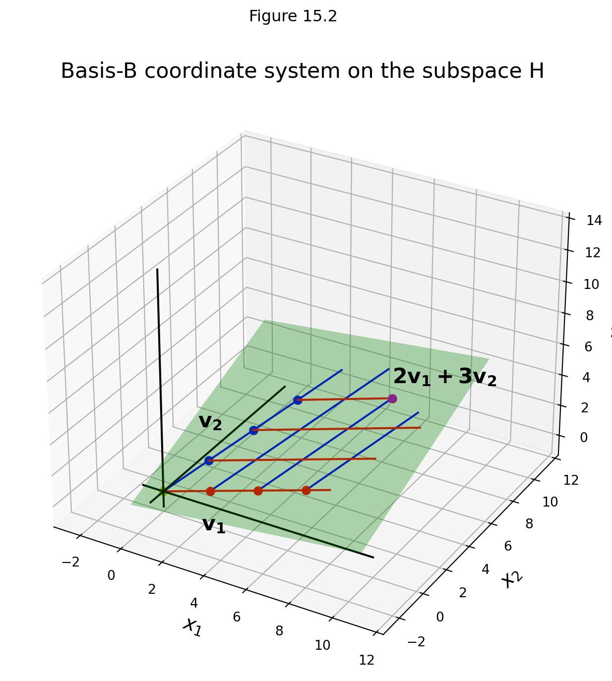
Let \(\mathbf{v}_1 = \begin{bmatrix}3\\6\\2\end{bmatrix}, \mathbf{v}_2 = \begin{bmatrix}-1\\0\\1\end{bmatrix}, \mathbf{x} = \begin{bmatrix}3\\12\\7\end{bmatrix},\) and \(\mathcal{B} = \{\mathbf{v}_1,\mathbf{v}_2\}.\)

Then \(\mathcal{B}\) is a basis for \(H\) = Span\(\{\mathbf{v}_1,\mathbf{v}_2\}\) because \(\mathbf{v}_1\) and \(\mathbf{v}_2\) are linearly independent.

Problem: Determine if \(\mathbf{x}\) is in \(H\), and if it is, find the coordinate vector of \(\mathbf{x}\) relative to \(\mathcal{B}.\)

Solution. If \(\mathbf{x}\) is in \(H,\) then the following vector equation is consistent:

\[\begin{split}c_1\begin{bmatrix}3\\6\\2\end{bmatrix} + c_2\begin{bmatrix}-1\\0\\1\end{bmatrix} = \begin{bmatrix}3\\12\\7\end{bmatrix}.\end{split}\]

The scalars \(c_1\) and \(c_2,\) if they exist, are the \(\mathcal{B}\)-coordinates of \(\mathbf{x}.\)

Row operations show that

\[\begin{split}\begin{bmatrix}3&-1&3\\6&0&12\\2&1&7\end{bmatrix} \sim \begin{bmatrix}1&0&2\\0&1&3\\0&0&0\end{bmatrix}.\end{split}\]

The reduced row echelon form shows that the system is consistent, so \(\mathbf{x}\) is in \(H\).

Furthermore, it shows that \(c_1 = 2\) and \(c_2 = 3,\)

so \([\mathbf{x}]_\mathcal{B} = \begin{bmatrix}2\\3\end{bmatrix}.\)

In this example, the basis \(\mathcal{B}\) determines a coordinate system on \(H\), which can be visualized like this:

Important: Don’t be confused by the fact that the “coordinate axes” are not purpendicular.

The whole idea here is that they don’t need to be.

As long as the independent vectors span the space, there is only one way to express any point in terms of them.

Thus, every point has a unique coordinate.

Isomorphism.

Another important idea is that, although points in \(H\) are in \(\mathbb{R}^3\), they are completely determined by their coordinate vectors, which belong to \(\mathbb{R}^2.\)

In our example, \(\begin{bmatrix}3\\12\\7\end{bmatrix}\mapsto\begin{bmatrix}2\\3\end{bmatrix}\).

We can see that the grid in the figure above makes \(H\) “look like” \(\mathbb{R}^2.\)

Note that a one-to-one correspondence is a function that is both one-to-one and onto – in other words, a bijection.

The correspondence \(\mathbf{x} \mapsto [\mathbf{x}]_\mathcal{B}\) is one-to-one correspondence between \(H\) and \(\mathbb{R}^2\) that preserves linear combinations.

In other words, if \(\mathbf{a} = \mathbf{b} + \mathbf{c}\) when \(\mathbf{a}, \mathbf{b}, \mathbf{c} \in H\),

then \([\mathbf{a}]_\mathcal{B} = [\mathbf{b}]_\mathcal{B} + [\mathbf{c}]_\mathcal{B}\) with \([\mathbf{a}]_\mathcal{B}, [\mathbf{b}]_\mathcal{B}, [\mathbf{c}]_\mathcal{B} \in \mathbb{R}^2\)

When we have a one-to-one correspondence between two subspaces that preserves linear combinations, we call such a correspondence an isomorphism, and we say that \(H\) is isomorphic to \(\mathbb{R}^2.\)

In general, if \(\mathcal{B}\ = \{\mathbf{b}_1,\dots,\mathbf{b}_p\}\) is a basis for \(H\), then the mapping \(\mathbf{x} \mapsto [\mathbf{x}]_\mathcal{B}\) is a one-to-one correspondence that makes \(H\) look and act the same as \(\mathbb{R}^p.\)

This is even through the vectors in \(H\) themselves may have more than \(p\) entries.

The Dimension of a Subspace

Here is an informal proof: Since \(H\) has a basis of \(p\) vectors, \(H\) is isomorphic to \(\mathbb{R}^p\). Any set consisting of more than \(p\) vectors in \(\mathbb{R}^p\) must be dependent. Recall that an isomorphism preserves vector relationships (sums, linear combinations, etc). So by the nature of an isomorphism, we can establish that any set of more than \(p\) vectors in \(H\) must be dependent. So any basis for \(H\) must have \(p\) vectors.

It can be shown that if a subspace \(H\) has a basis of \(p\) vectors, then every basis of \(H\) must consist of exactly \(p\) vectors.

That is, for a given \(H\), the number \(p\) is a special number.

Thus we can make this definition:

Definition. The dimension of a nonzero subspace \(H,\) denoted by \(\dim H,\) is the number of vectors in any basis for \(H.\)

The dimension of the zero subspace \(\{{\bf 0}\}\) is defined to be zero.

So now we can say with precision things we’ve previous said informally.

For example, a plane through \({\bf 0}\) is two-dimensional, and a line through \({\bf 0}\) is one-dimensional.

Question: What is the dimension of a line not through the origin?

Answer: It is undefined, because a line not through the the origin is not a subspace, so cannot have a basis, so does not have a dimension.

Dimension of the Null Space

At the end of the last lecture we looked at this matrix:

\[\begin{split}A = \begin{bmatrix}-3&6&-1&1&-7\\1&-2&2&3&-1\\2&-4&5&8&-4\end{bmatrix}\end{split}\]

We determined that its null space had a basis consisting of 3 vectors.

So the dimension of \(A\)’s null space (ie, \(\dim\operatorname{Nul} A\)) is 3.

Remember that we constructed an explicit description of the null space of this matrix, as:

\[\begin{split} = x_2\begin{bmatrix}2\\1\\0\\0\\0\end{bmatrix}+x_4\begin{bmatrix}1\\0\\-2\\1\\0\end{bmatrix}+x_5\begin{bmatrix}-3\\0\\2\\0\\1\end{bmatrix} \end{split}\]

Each basis vector corresponds to a free variable in the equation \(A\mathbf{x} = {\bf 0}.\)

So, to find the dimension of \(\operatorname{Nul}\ A,\) simply identify and count the number of free variables in \(A\mathbf{x} = {\bf 0}.\)

Matrix Rank

Definition. The rank of a matrix, denoted by \(\operatorname{Rank} A,\) is the dimension of the column space of \(A\).

Since the pivot columns of \(A\) form a basis for \(\operatorname{Col} A,\) the rank of \(A\) is just the number of pivot columns in \(A\).

Example. Determine the rank of the matrix

\[\begin{split}A = \begin{bmatrix}2&5&-3&-4&8\\4&7&-4&-3&9\\6&9&-5&2&4\\0&-9&6&5&-6\end{bmatrix}.\end{split}\]

Solution Reduce \(A\) to an echelon form:

\[\begin{split}A = \begin{bmatrix}2&5&-3&-4&8\\0&-3&2&5&-7\\0&-6&4&14&-20\\0&-9&6&5&-6\end{bmatrix}\sim\cdots\sim\begin{bmatrix}2&5&-3&-4&8\\0&-3&2&5&-7\\0&0&0&4&-6\\0&0&0&0&0\end{bmatrix}.\end{split}\]

The matrix \(A\) has 3 pivot columns, so \(\operatorname{Rank} A = 3.\)

The Rank Theorem

Consider a matrix \(A.\)

In the last lecture we showed the following: one can construct a basis for \(\operatorname{Nul} A\) using the columns corresponding to free variables in the solution of \(A\mathbf{x} = {\bf 0}.\)

This shows that \(\dim\operatorname{Nul} A\) = the number of free variables in \(A\mathbf{x} = {\bf 0},\)

which is the number of non-pivot columns in \(A\).

We also saw that the number of columns in any basis for \(\operatorname{Col}\ A\) is the number of pivot columns.

So we can now make this important connection:

\[\begin{split}\begin{array}{rcl} \dim\operatorname{Nul} A + \dim\operatorname{Col} A &= &\mbox{number of non-pivot columns of $A$ + number of pivot columns of $A$}\\ &= &\mbox{number of columns of $A$}. \end{array}\end{split}\]

This leads to the following theorem:

Theorem. If a matrix \(A\) has \(n\) columns, then \(\operatorname{Rank} A + \dim\operatorname{Nul} A = n\).

This is a terrifically important fact!

Here is an intuitive way to understand it. Let’s think about a matrix \(A\) and the associated linear transformation \(T(x) = Ax\).

If the matrix \(A\) has \(n\) columns, then \(A\)’s column space could have dimension as high as \(n\).

In other words, \(T\)’s range could have dimension as high as \(n\).

However, if \(A\) “throws away” a nullspace of dimension \(p\), then that reduces the columnspace of \(A\) to \(n-p\).

Meaning, the dimension of \(T\)’s range is reduced to \(n-p\).

Extending the Invertible Matrix Theorem

The above arguments show that when \(A\) has \(n\) columns, then the “larger” that the column space is, the “smaller” that the null space is.

(Where “larger” means “has more dimensions.”)

This is particularly important when \(A\) is square \((n\times n)\).

Let’s consider the extreme, in which the column space of \(A\) has maximum dimension – i.e., \(\dim\operatorname{Col}\ A= n.\)

Recall that the IMT said that an \(n\times n\) matrix is invertible if and only if its columns are linearly independent, and if and only if its columns span \(\mathbb{R}^n.\)

Hence we now can see that an \(n\times n\) matrix is invertible if and only if the columns of \(A\) form a basis for \(\mathbb{R}^n.\)

This leads to the following facts, which further extend the IMT:

Let \(A\) be an \(n\times n\) matrix. Then the following statements are each equivalent to the statement that \(A\) is an invertible matrix:

1. The columns of \(A\) form a basis for \(\mathbb{R}^n.\)

2. \(\operatorname{Col} A = \mathbb{R}^n.\)

3. \(\dim\operatorname{Col} A = n.\)

4. \(\operatorname{Rank} A = n.\)

5. \(\operatorname{Nul} A = \{{\bf 0}\}.\)

6. \(\dim\operatorname{Nul} A = 0.\)