Show code cell source Hide code cell source

import numpy as np
import scipy as sp
import matplotlib.pyplot as plt
import pandas as pd
import seaborn as sns
import matplotlib as mp
import sklearn
from IPython.display import Image, HTML

import laUtilities as ut

%matplotlib inline

Recommender Systems

Today, we look at a topic that has become enormously important in society: recommender systems.

We will

• Define recommender systems

• Review the challenges they pose

• Discuss two classic methods:

  • Collaborative Filtering

  • Matrix Factorization

Note

This section draws heavily on

• These slides by Alex Smola

• Matrix Factorization Techniques for Recommender Systems, by Yehuda Koren, Robert Bell, and Chris Volinsky, and

• Collaborative Filtering with Temporal Dynamics, by Yehuda Koren

What are Recommender Systems?

The concept of recommender systems emerged in the late 1990s / early 2000s as social life moved online:

• online purchasing and commerce

• online discussions and ratings

• social information sharing

In these systems content was exploding and users were having a hard time finding things they were interested in.

Users wanted recommendations.

Over time, the problem has only gotten worse:

An enormous need has emerged for systems to help sort through products, services, and content items.

This often goes by the term personalization.

Some examples:

• Movie recommendation (Netflix, YouTube)

• Related product recommendation (Amazon)

• Web page ranking (Google)

• Social content filtering (Facebook, Twitter)

• Services (Airbnb, Uber, TripAdvisor)

• News content recommendation (Apple News)

• Priority inbox & spam filtering (Google)

• Online dating (OK Cupid)

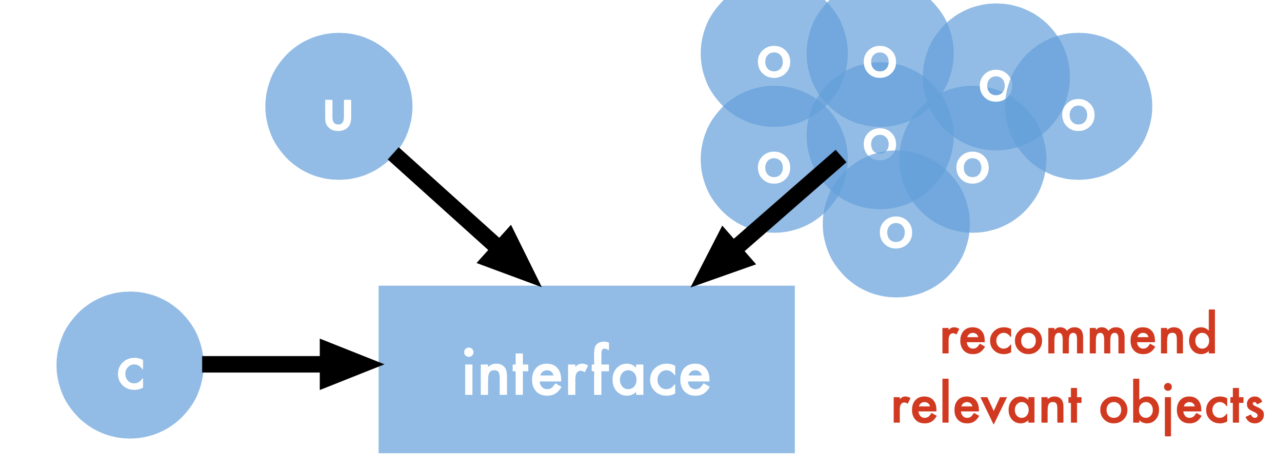
A more formal view:

• User - requests content

• Objects - that can be displayed

• Context - device, location, time

• Interface - browser, mobile

Inferring Preferences

Unfortunately, users generally have a hard time explaining what types of content they prefer. Some early systems worked by interviewing users to ask what they liked. Those systems did not work very well.

Note

A very interesting article about the earliest personalization systems is User Modeling via Stereotypes by Elaine Rich, dating from 1979.

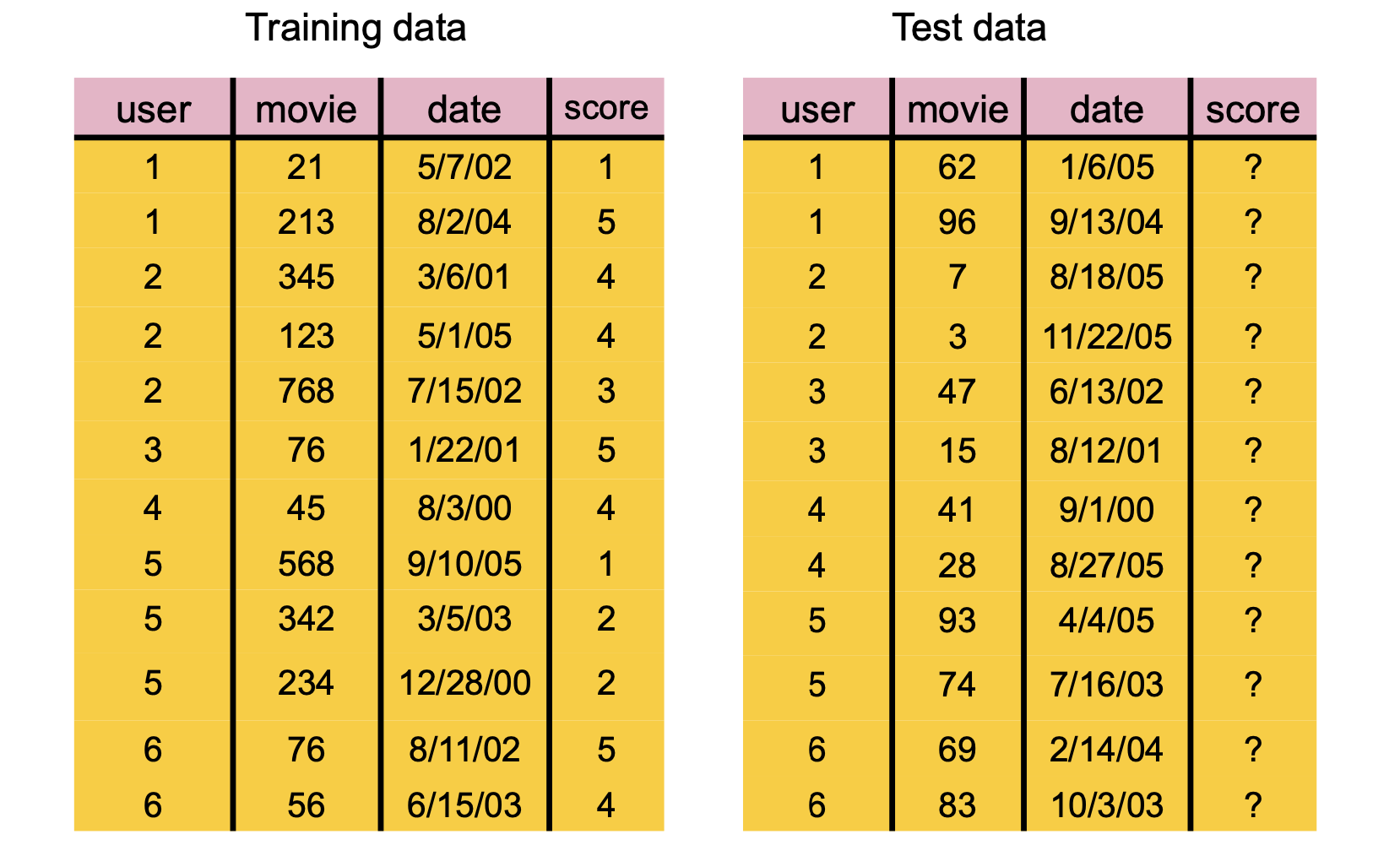
Instead, modern systems work by capturing user’s opinions about specific items.

This can be done actively:

• When a user is asked to rate a movie, product, or experience,

Or it can be done passively:

• By noting which items a user chooses to purchase (for example).

Challenges

• The biggest issue is scalability: typical data for this problem is huge.

  • Millions of objects

  • 100s of millions of users

• Changing user base

• Changing inventory (movies, stories, goods)

• Available features

• Imbalanced dataset

  • User activity / item reviews are power law distributed

Note

This data is a subset of the data presented in: “From amateurs to connoisseurs: modeling the evolution of user expertise through online reviews,” by J. McAuley and J. Leskovec. WWW, 2013

Show code cell content Hide code cell content

# This is a 1.7 GB file, delete it after use
import os.path
if not os.path.exists('train.csv'):
    os.system('kaggle competitions download -c cs-506-midterm-a1-b1')
    os.system('unzip cs-506-midterm-a1-b1.zip')

df = pd.read_csv('train.csv')

Show code cell content Hide code cell content

n_users = df["UserId"].unique().shape[0]
n_movies = df["ProductId"].unique().shape[0]
n_reviews = len(df)
print(f'There are {n_reviews} reviews, {n_movies} movies and {n_users} users.')
print(f'There are {n_users * n_movies} potential reviews, meaning sparsity of {(n_reviews/(n_users * n_movies)):0.4%}')

There are 1697533 reviews, 50052 movies and 123960 users.
There are 6204445920 potential reviews, meaning sparsity of 0.0274%

Reviews are Sparse.

Example: A commonly used dataset for testing consists of Amazon movie reviews:

• 1,697,533 reviews

• 123,960 users

• 50,052 movies

Notice that there are 6,204,445,920 potential reviews, but we only have 1,697,533 actual reviews.

Only 0.02% of the reviews are available – 99.98% of the reviews are missing.

Show code cell source Hide code cell source

print(f'There are on average {n_reviews/n_movies:0.1f} reviews per movie' +
     f' and {n_reviews/n_users:0.1f} reviews per user')

There are on average 33.9 reviews per movie and 13.7 reviews per user

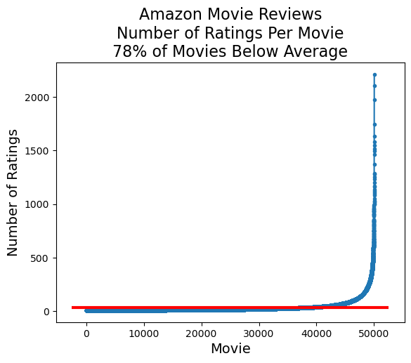
Sparseness is skewed.

Although on average a movie receives 34 reviews, almost all movies have even fewer reviews.

Show code cell source Hide code cell source

reviews_per_movie = df.groupby('ProductId').count()['Id'].values
frac_below_mean = np.sum(reviews_per_movie < (n_reviews/n_movies))/len(reviews_per_movie)
plt.plot(sorted(reviews_per_movie), '.-')
xmin, xmax, ymin, ymax = plt.axis()
plt.hlines(n_reviews/n_movies, xmin, xmax, 'r', lw = 3)
plt.ylabel('Number of Ratings', fontsize = 14)
plt.xlabel('Movie', fontsize = 14)
plt.title(f'Amazon Movie Reviews\nNumber of Ratings Per Movie\n' +
          f'{frac_below_mean:0.0%} of Movies Below Average', fontsize = 16);

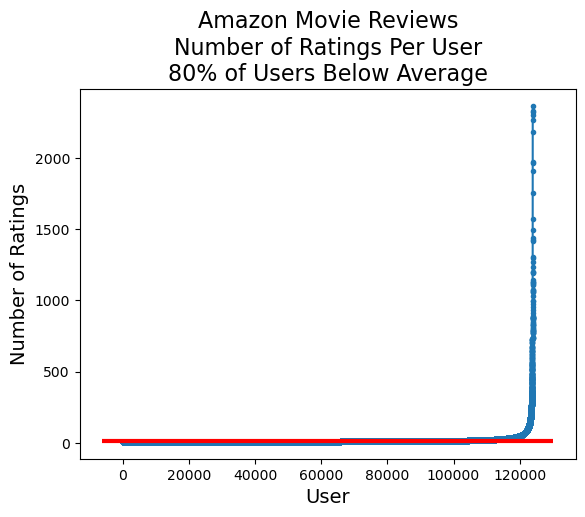
Likewise, although the average user writes 14 reviews, almost all users write even fewer reviews.

Show code cell source Hide code cell source

reviews_per_user = df.groupby('UserId').count()['Id'].values
frac_below_mean = np.sum(reviews_per_user < (n_reviews/n_users))/len(reviews_per_user)
plt.plot(sorted(reviews_per_user), '.-')
xmin, xmax, ymin, ymax = plt.axis()
plt.hlines(n_reviews/n_users, xmin, xmax, 'r', lw = 3)
plt.ylabel('Number of Ratings', fontsize = 14)
plt.xlabel('User', fontsize = 14)
plt.title(f'Amazon Movie Reviews\nNumber of Ratings Per User\n' +
          f'{frac_below_mean:0.0%} of Users Below Average', fontsize = 16);

A typical objective function is root mean square error (RMSE)

\[ \text{RMSE} = \sqrt{1/|S| \sum_{(i,u)\in S} (\hat{r}_{ui} - r_{ui})^2} \]

where \( r_{ui} \) is the rating that user \(u\) gives to item \(i\), and \(S\) is the set of all ratings.

OK, now we know the problem and the data available. How can we address the problem?

The earliest method developed is called collaborative filtering.

Collaborative Filtering

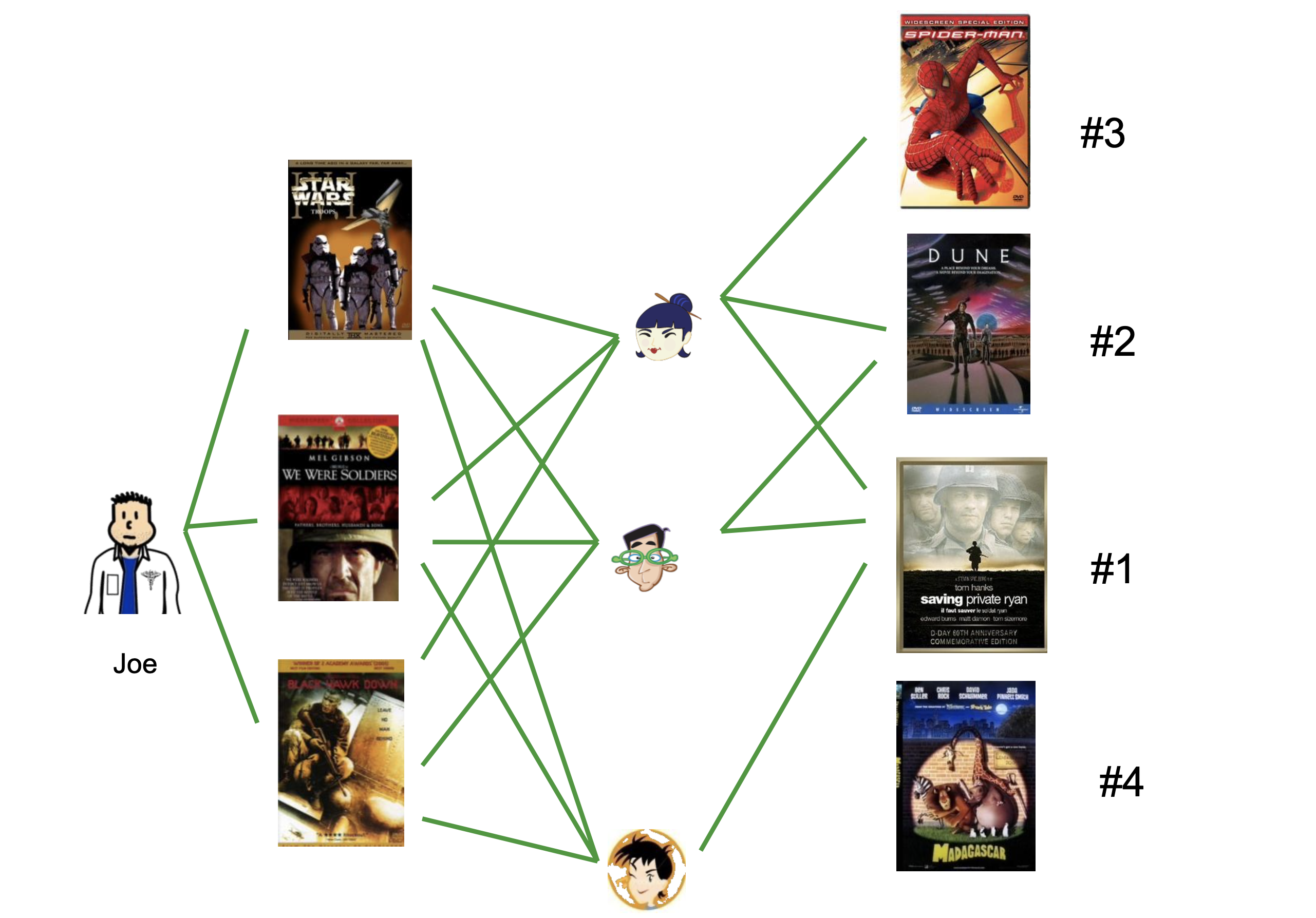
The central idea of collaborative filtering is that the set of known recommendations can be considered to be a bipartite graph.

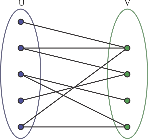
The nodes of the bipartite graph are users and items.

Each edge corresponds to a known rating \(r_{ui}.\)

Then recommendations are formed by traversing or processing the bipartite graph.

There are at least two ways this graph can be used.

To form a rating for item \((u, i)\):

1. Using user-user similarity:

   • look at users that have similar item preferences to user \(u\)

   • look at how those users rated item \(i\)

Good for many users, fewer items

2. Using item-item similarity:

   • look at other items that have been liked by similar users as item \(i\)

   • look at how user \(u\) rated those items

Good for many items, fewer users

Item-item CF

Let’s look at the item-item CF approach in detail.

The questions are:

• How do we judge “similarity” of items?

• How do we form a predicted rating?

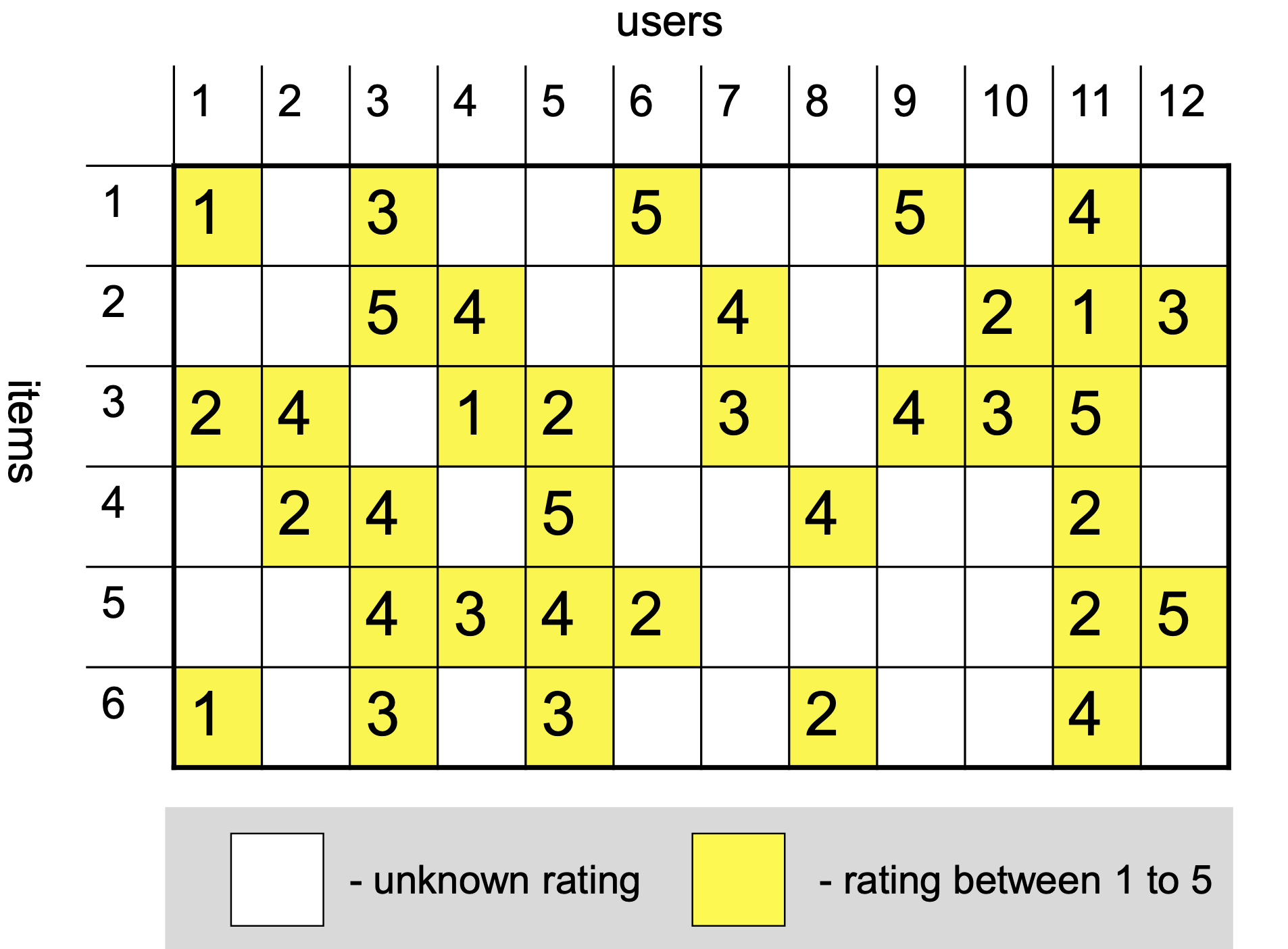
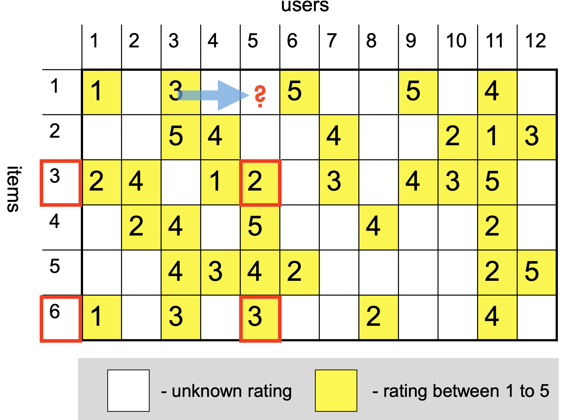
Here is another view of the ratings graph, this time as a matrix that includes missing entries:

Let’s say we want to predict the value of this unknown rating:

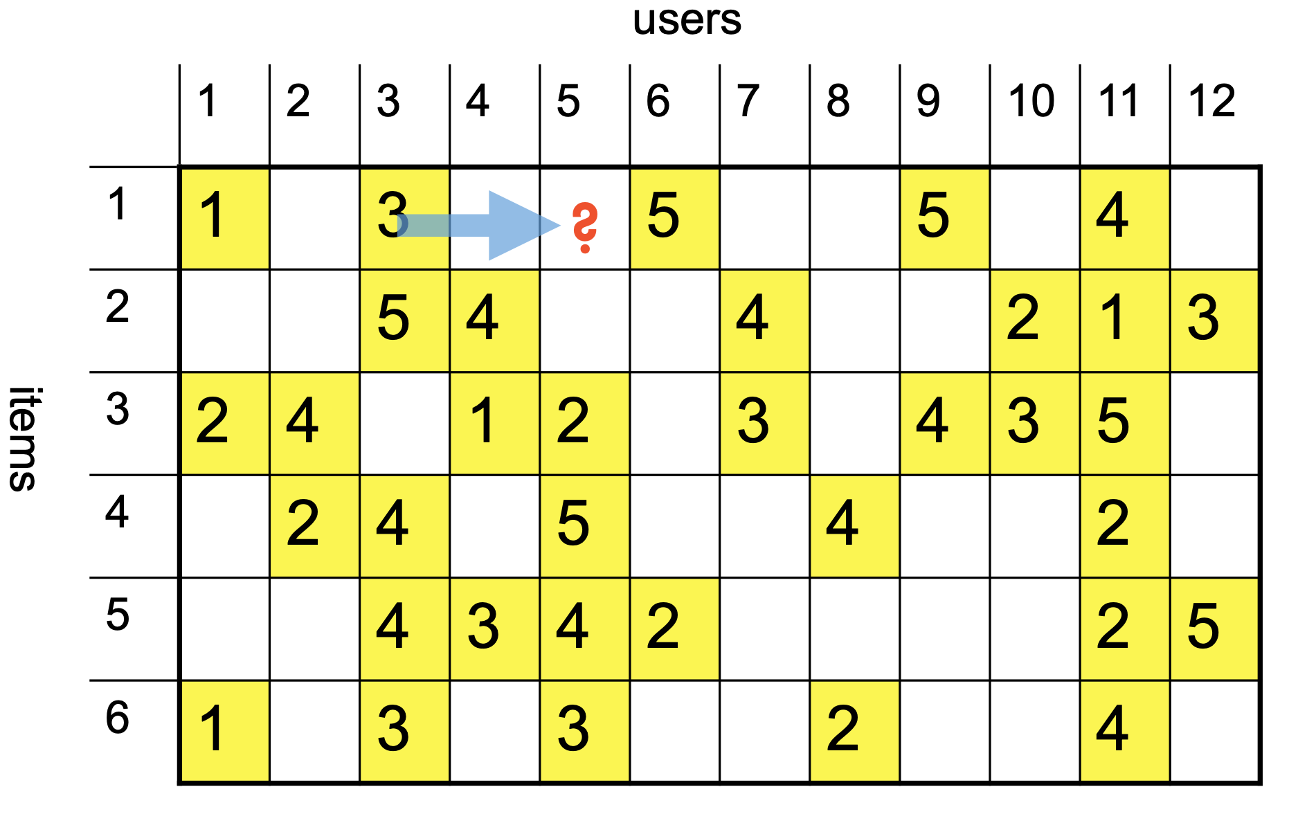
We’ll consider two other items, namely items 3 and 6 (for example).

Note that we are only interested in items that this user has rated.

We will discuss strategies for assessing similarity shortly.

How did we choose these two items?

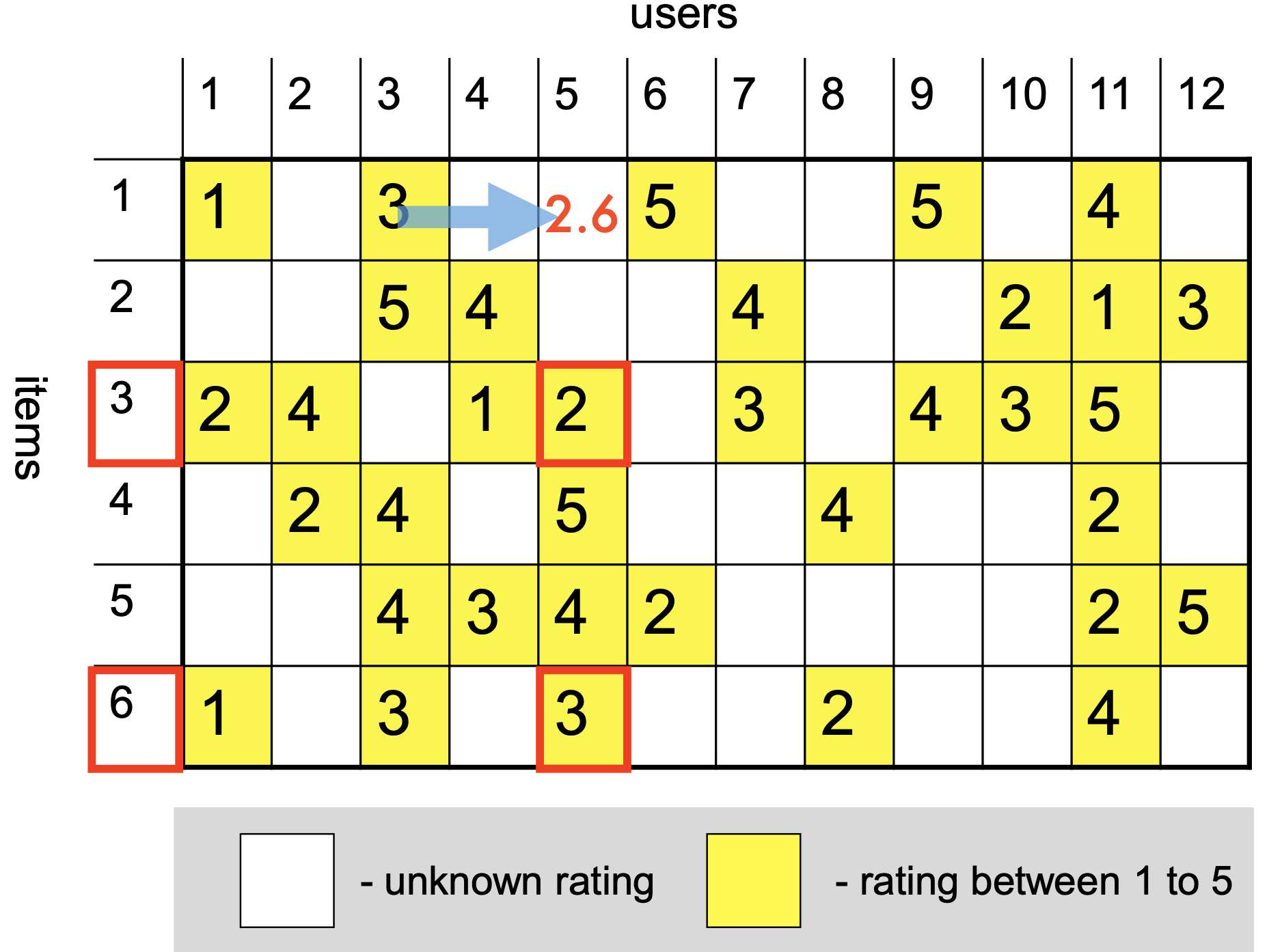
We used \(k\)-nearest neighbors. Here \(k\) = 2.

For now, let’s just say we determine the similarities as:

\[ s_{13} = 0.2 \]

\[ s_{16} = 0.3 \]

These similarity scores tell us how much weight to put on the rating of the other items.

So we can form a prediction of \(\hat{r}_{15}\) as:

\[ \hat{r}_{15} = \frac{s_{13} \cdot r_{35} + s_{16} \cdot r_{65}}{s_{13} + s_{16}} = \frac{0.2 \cdot 2 + 0.3 \cdot 3}{0.2 + 0.3} = 2.6 \]

Similarity

How should we assess similarity of items?

A reasonable approach is to consider items similar if their ratings are correlated.

So we can use the Pearson correlation coefficient \(r\).

However, note that two items will not have ratings in the same positions.

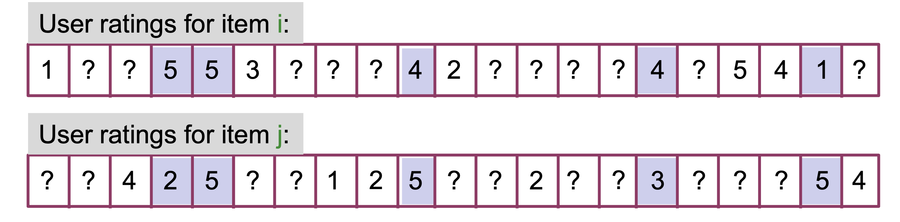
So we want to compute correlation only over the users who rated both the items.

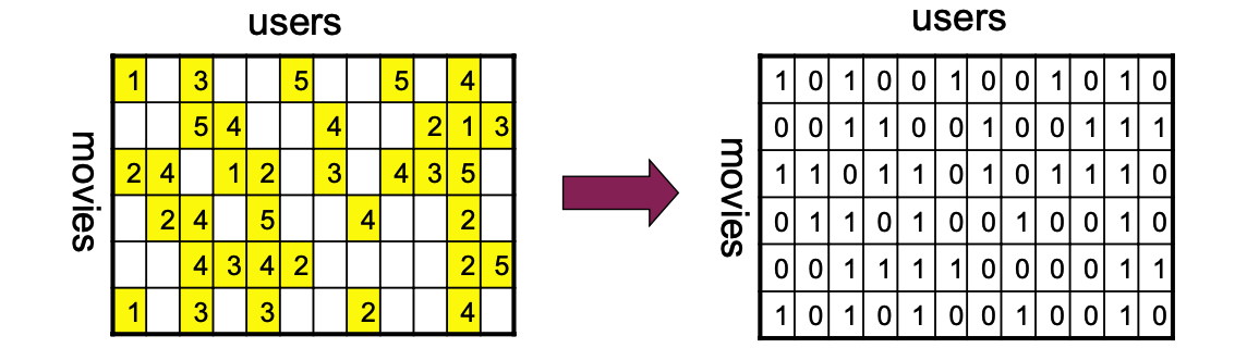
In some cases we will need to work with binary \(r_{ui}\)s.

For example, purchase histories on an e-commerce site, or clicks on an ad.

In this case, an appropriate replacement for Pearson \(r\) is the Jaccard similarity coefficient.

(See the lecture on similarity measures.)

Improving CF

One problem with the story so far arises due to bias.

• Some items are significantly higher or lower rated

• Some users rate substantially higher or lower in general

These properties interfere with similarity assessment.

Bias correction is crucial for CF recommender systems.

We need to include

• Per-user offset

• Per-item offset

• Global offset

Hence we need to form a per-item bias of:

\[ b_{ui} = \mu + \alpha_u + \beta_i \]

where \(\alpha_u\) is the per-user offset of user \(u\) and \(\beta_i\) is the per-item offset of item \(i\).

How can we estimate the \(\alpha\)s, the \(\beta\)s, and the \(\mu\)?

Let’s assume for a minute that we had a fully-dense matrix of ratings \(R\).

\(R\) has items on the rows and users on the columns.

Then what we want to estimate is

\[\min_{\alpha,\beta,\mu} \Vert R - \mathbf{1}\alpha^T + \beta\mathbf{1}^T + \mu1\Vert^2 + \lambda(\Vert\alpha\Vert^2 + \Vert\beta\Vert^2) \]

Here, \(\mathbf{1}\) represents appropriately sized vectors of ones, and \(1\) is a matrix of ones.

While this is not a simple ordinary least squares problem, there is a strategy for solving it.

Assume we hold \(\beta\mathbf{1}^T + \mu1\) constant.

Then the remaining problem is

\[\min_{\alpha} \Vert R - \mathbf{1}\alpha^T \Vert^2 + \lambda \Vert\alpha\Vert^2 \]

which (for each column of \(R\)) is a standard least squares problem (which we solve via Ridge regression).

This sort of problem is called jointly convex.

The strategy for solving is:

1. Hold \(\alpha\) and \(\beta\) constant, solve for \(\mu\).

2. Hold \(\alpha\) and \(\mu\) constant, solve for \(\beta\).

3. Hold \(\beta\) and \(\mu\) constant, solve for \(\alpha\).

Each of the three steps will reduce the overall error. So we iterate over them until convergence.

The last issue is that the matrix \(R\) is not dense - in reality we only have a small subset of its entries.

We simply need to adapt the least-squares solution to only consider the entries in \(R\) that we know.

As a result, the actual calculation is:

Step 1:

\[ \mu = \frac{\sum_{(u, i) \in R} (r_{ui} - \alpha_u - \beta_i)}{|R|} \]

Step 2:

\[ \alpha_u = \frac{\sum_{i \in R(u)}(r_{ui} - \mu - \beta_i)}{\lambda + |R(u)|} \]

Step 3:

\[ \beta_i = \frac{\sum_{u \in R(i)}(r_{ui} - \mu - \alpha_u)}{\lambda + |R(i)|} \]

Step 4: If not converged, go to Step 1.

Now that we have the biases learned, we can do a better job of estimating correlation:

\[ \hat{\rho}_{ij} = \frac{\sum_{u\in U(i,j)}(r_{ui} - b_{ui})(r_{uj}-b_{uj})} {\sqrt{\sum_{u\in U(i,j)}(r_{ui} - b_{ui})^2\sum_{u\in U(i,j)}(r_{uj}-b_{uj})^2}} \]

where

• \(b_{ui} = \mu + \alpha_u + \beta_i\), and

• \(U(i,j)\) are the users who have rated both \(i\) and \(j\).

And using biases we can also do a better job of estimating ratings:

\[ \hat{r}_{ui} = b_{ui} + \frac{\sum_{j \in n_k(i, u)} s_{ij}(r_{uj} - b_{uj})}{\sum_{j \in n_k(i, u)} s_{ij}} \]

where

• \(b_{ui} = \mu + \alpha_u + \beta_i\), and

• \(n_k(i, u)\) are the \(k\) nearest neighbors to \(i\) that were rated by user \(u\).

Assessing CF

This completes the high level view of CF.

Working with user-user similarities is analogous.

Strengths:

• Essentially no training.

  • The reliance on \(k\)-nearest neighbors helps in this respect.

• Easy to update with new users, items, and ratings

• Can be explained to user:

  • “We recommend Minority Report because you liked Blade Runner and Total Recall.”

Weaknesses:

• Accuracy can be a problem

• Scalability can be a problem (think \(k\)-NN)

Matrix Factorization

Note that standard CF forces us to consider similarity among items, or among users, but does not take into account both.

Can we use both kinds of similarity simultaneously?

We can’t use both the rows and columns of the ratings matrix \(R\) at the same time – the user and item vectors live in different vector spaces.

What we could try to do is find a single vector space in which we represent both users and items, along with a similarity function, such that:

• users who have similar item ratings are similar in the vector space

• items who have similar user ratings are similar in the vector space

• when a given user highly rates a given item, that user and item are similar in the vector space.

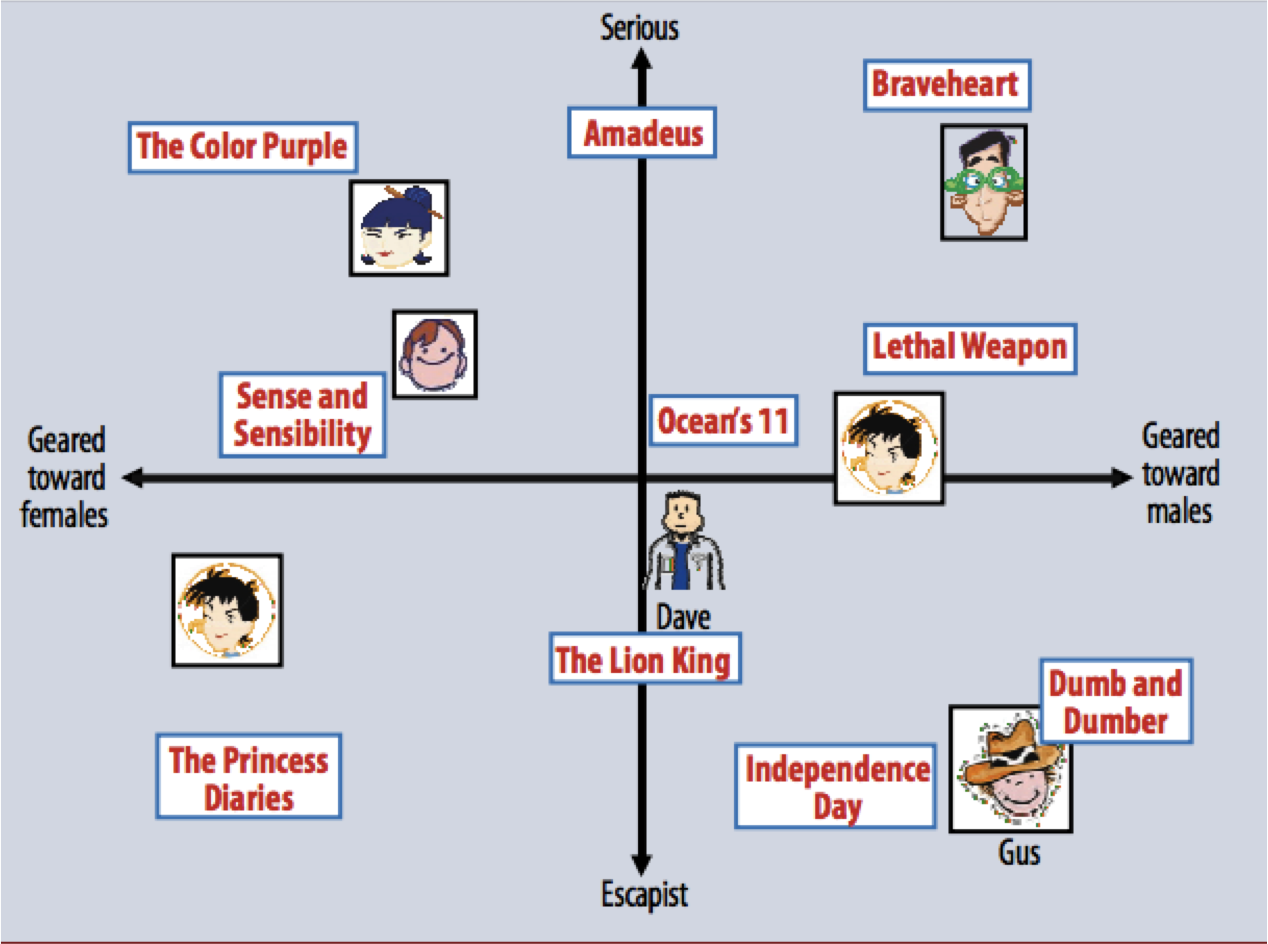
Koren et al, IEEE Computer, 2009

We saw this idea previously, in an SVD lecture.

This new vector space is called a latent space,

and the user and item representations are called latent vectors.

Now, however, we are working with a matrix which is only partially observed.

That is, we only know some of the entries in the ratings matrix.

Nonetheless, we can imagine a situation like this:

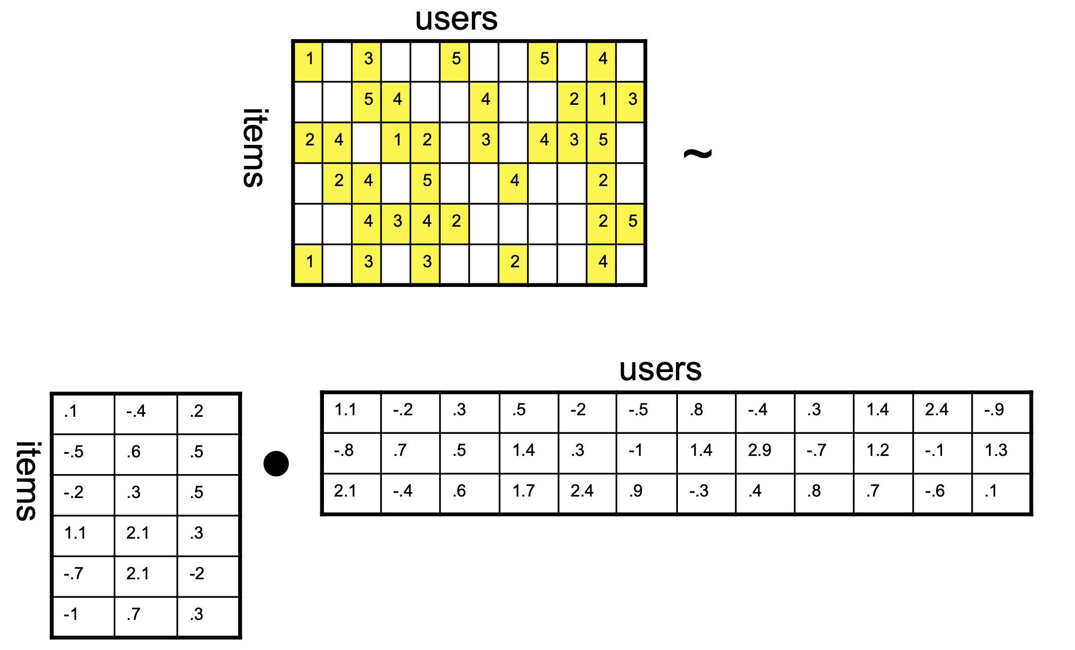
Now we want the product of the two matrices on the right to be as close as possible to the known values of the ratings matrix.

What this setup implies is that our similarity function is the inner product.

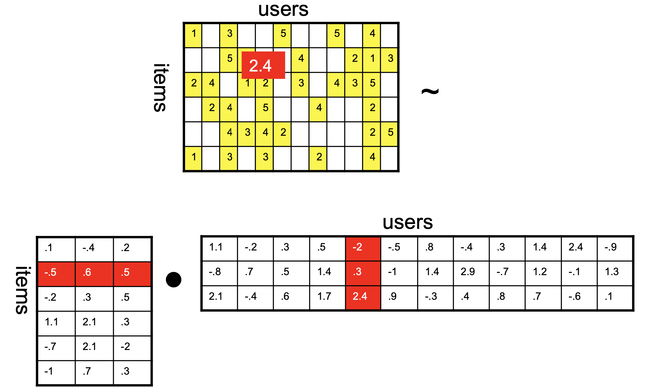
Which means that to predict an unknown rating, we take the inner product of latent vectors:

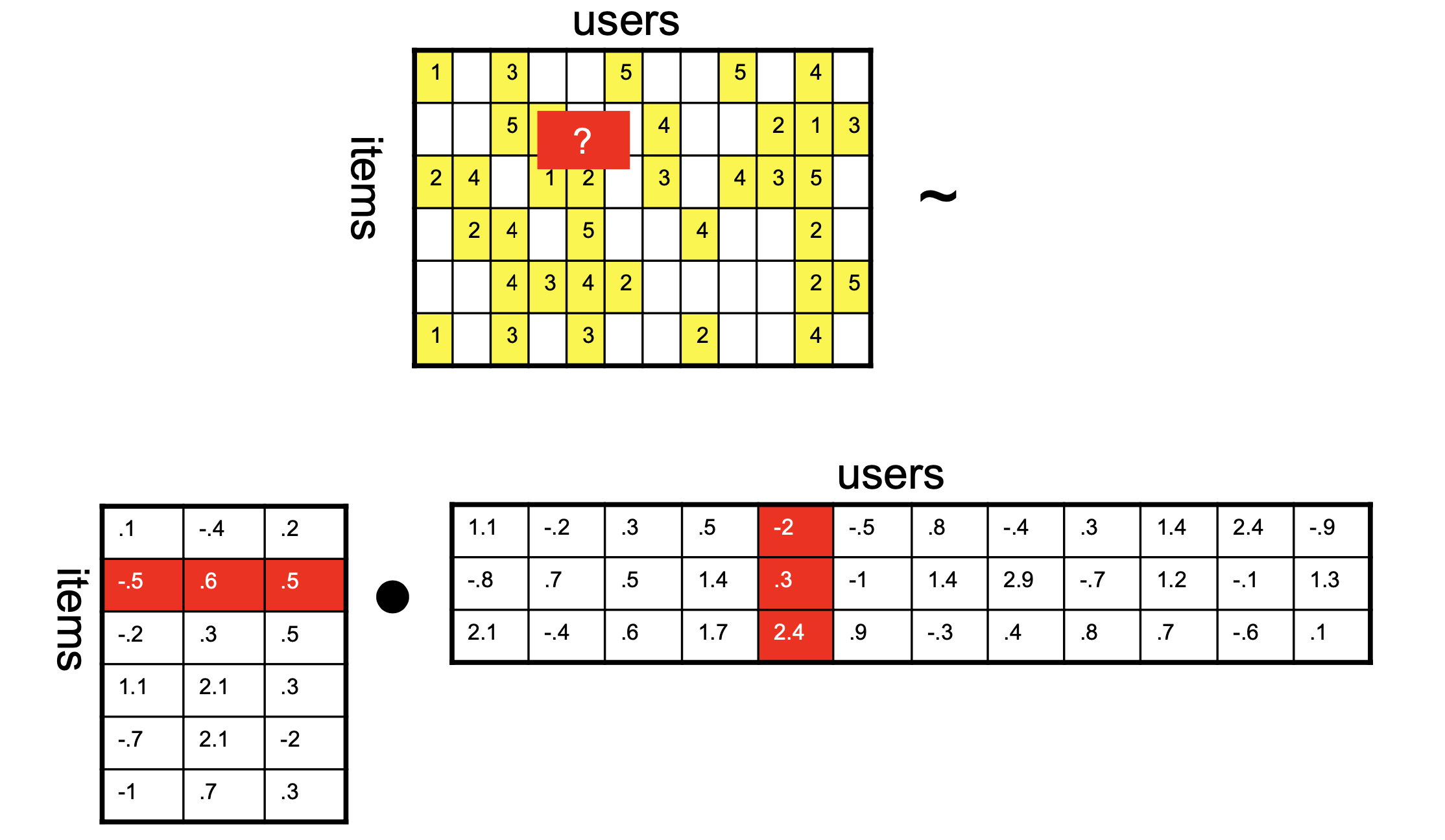
Now \((-2 \cdot -0.5)+(0.3 \cdot 0.6)+(2.5 \cdot 0.5) = 2.43\), so:

Solving Matrix Factorization

Notice that in this case we’ve decided that the factorization should be rank 3, ie, low-rank.

So we want something like an SVD.

(Recall that SVD gives us the most-accurate-possible low-rank factorization of a matrix).

However, we can’t use the SVD algorithm directly, because we don’t know all the entries in \(R\).

(Indeed, the unseen entries in \(R\) as exactly what we want to predict.)

Here is what we want to solve:

\[ \min_{U,V} \Vert (R - UV^T)_S\Vert^2 + \lambda(\Vert U\Vert^2 + \Vert V\Vert^2) \]

where \(R\) is \(m\times n\), \(U\) is the \(m\times k\) items matrix and \(V\) is the \(n\times k\) users matrix.

The \((\cdot)_S\) notation means that we are only considering the matrix entries that correspond to known reviews (the set \(S\)).

Note that as usual, we add \(\ell_2\) penalization to avoid overfitting (Ridge regression).

Once again, this problem is jointly convex.

In particular, it we hold either \(U\) or \(V\) constant, then the result is a simple ridge regression.

So one commonly used algorithm for this problem is called alternating least squares:

1. Hold \(U\) constant, and solve for \(V\)

2. Hold \(V\) constant, and solve for \(U\)

3. If not converged, go to Step 1.

The only thing I’ve left out at this point is how to deal with the missing entries of \(R\).

It’s not hard, but the details aren’t that interesting, so I will give you code instead!

ALS in Practice

The entire Amazon reviews dataset is too large to work with easily, and it is too sparse.

Hence, we will take the densest rows and columns of the matrix.

# The densest columns: products with more than 50 reviews
pids = df.groupby('ProductId').count()['Id']
hi_pids = pids[pids > 50].index

# reviews that are for these products
hi_pid_rec = [r in hi_pids for r in df['ProductId']]

# the densest rows: users with more than 50 reviews
uids = df.groupby('UserId').count()['Id']
hi_uids = uids[uids > 50].index

# reviews that are from these users
hi_uid_rec = [r in hi_uids for r in df['UserId']]

# reviews that are from those users and for those movies
goodrec = [a and b for a, b in zip(hi_uid_rec, hi_pid_rec)]

Now we create a matrix from these reviews.

Missing entries will be filled with NaNs.

dense_df = df.loc[goodrec]
good_df = dense_df.loc[~df['Score'].isnull()]
R = good_df.pivot_table(columns = 'ProductId', index = 'UserId', values = 'Score')

R

ProductId	0005019281	0005119367	0307142485	0307142493	0307514161	0310263662	0310274281	0718000315	0764001035	0764003828	...	B00IKM5OCO	B00IWULQQ2	B00J4LMHMK	B00J5JSV1W	B00JA3RPAG	B00JAQJMJ0	B00JBBJJ24	B00JKPHUE0	B00K2CHVJ4	B00L4IDS4W
UserId
A02755422E9NI29TCQ5W3	NaN	NaN	NaN	NaN	NaN	NaN	NaN	NaN	NaN	NaN	...	NaN	NaN	NaN	NaN	NaN	NaN	NaN	NaN	NaN	NaN
A100JCBNALJFAW	NaN	NaN	NaN	NaN	NaN	NaN	NaN	NaN	NaN	NaN	...	NaN	NaN	NaN	NaN	NaN	NaN	NaN	NaN	NaN	NaN
A10175AMUHOQC4	NaN	NaN	NaN	NaN	NaN	NaN	NaN	NaN	NaN	NaN	...	NaN	NaN	NaN	NaN	NaN	NaN	NaN	NaN	NaN	NaN
A103KNDW8GN92L	NaN	NaN	NaN	NaN	NaN	4.0	NaN	NaN	NaN	NaN	...	NaN	NaN	NaN	NaN	NaN	NaN	NaN	NaN	NaN	NaN
A106016KSI0YQ	NaN	NaN	NaN	NaN	NaN	NaN	NaN	NaN	NaN	NaN	...	NaN	NaN	NaN	NaN	NaN	NaN	NaN	NaN	NaN	NaN
...	...	...	...	...	...	...	...	...	...	...	...	...	...	...	...	...	...	...	...	...	...
AZUBX0AYYNTFF	NaN	NaN	NaN	NaN	NaN	NaN	NaN	NaN	NaN	NaN	...	NaN	NaN	NaN	NaN	NaN	NaN	NaN	NaN	NaN	NaN
AZXGPM8EKSHE9	NaN	NaN	NaN	NaN	NaN	NaN	NaN	NaN	NaN	NaN	...	NaN	NaN	NaN	NaN	NaN	NaN	NaN	NaN	NaN	NaN
AZXHK8IO25FL6	NaN	NaN	NaN	NaN	NaN	NaN	NaN	NaN	NaN	NaN	...	NaN	NaN	NaN	NaN	NaN	NaN	NaN	NaN	NaN	NaN
AZXR5HB99P936	NaN	NaN	NaN	NaN	NaN	NaN	NaN	NaN	NaN	NaN	...	NaN	NaN	NaN	NaN	NaN	NaN	NaN	NaN	NaN	NaN
AZZ4GD20C58ND	NaN	NaN	NaN	NaN	NaN	NaN	NaN	NaN	NaN	NaN	...	NaN	NaN	NaN	NaN	NaN	NaN	NaN	NaN	NaN	NaN

3677 rows × 7244 columns

import MF as MF

# I am pulling these hyperparameters out of the air;
# That's not the right way to do it!
RS = MF.als_MF(rank = 20, lambda_ = 1)

%time pred, error = RS.fit_model(R)

CPU times: user 11min 1s, sys: 24min 30s, total: 35min 32s
Wall time: 3min 52s

Show code cell source Hide code cell source

print(f'RMSE on visible entries (training data): {np.sqrt(error/R.count().sum()):0.3f}')

RMSE on visible entries (training data): 0.344

pred

ProductId	0005019281	0005119367	0307142485	0307142493	0307514161	0310263662	0310274281	0718000315	0764001035	0764003828	...	B00IKM5OCO	B00IWULQQ2	B00J4LMHMK	B00J5JSV1W	B00JA3RPAG	B00JAQJMJ0	B00JBBJJ24	B00JKPHUE0	B00K2CHVJ4	B00L4IDS4W
UserId
A02755422E9NI29TCQ5W3	5.214071	5.337271	5.056362	4.087416	5.407318	5.297832	5.071851	4.281667	4.749674	4.973165	...	3.650950	5.014452	4.495824	3.159308	4.592631	4.737402	4.844146	4.857948	3.970947	4.807057
A100JCBNALJFAW	4.417716	3.817517	3.224885	2.357864	5.030919	2.621849	3.948541	3.346081	3.728381	2.551108	...	3.829715	3.925485	3.231605	3.145845	4.113032	4.462769	2.925964	2.396574	2.887802	3.132729
A10175AMUHOQC4	5.293009	4.997519	5.887083	5.469588	4.961311	4.931874	4.692830	3.581315	4.272003	4.683869	...	4.230151	4.732049	5.258265	2.890735	4.361825	5.417988	6.094052	4.464990	4.183745	4.107988
A103KNDW8GN92L	4.507828	4.936013	4.201449	6.079262	4.308772	3.876277	4.287324	4.428760	4.306389	5.911843	...	3.694592	4.522997	5.072133	2.288274	3.707725	4.664537	4.901905	4.725056	4.371643	4.125607
A106016KSI0YQ	3.845861	4.375542	2.865917	4.754560	4.615124	3.731579	4.204170	3.166638	3.870211	4.389759	...	4.158656	3.886184	2.773142	2.501356	2.541995	3.564672	3.943119	2.447221	2.340907	1.915349
...	...	...	...	...	...	...	...	...	...	...	...	...	...	...	...	...	...	...	...	...	...
AZUBX0AYYNTFF	3.674328	4.317386	3.246379	4.588257	4.433596	3.773535	3.810215	3.088035	2.628883	3.896187	...	2.849555	3.482059	2.862210	1.798721	2.512885	4.537965	3.276120	3.582396	2.254772	2.610681
AZXGPM8EKSHE9	2.622713	3.290833	0.960872	3.759832	3.664305	3.286624	3.864391	3.333899	3.396193	1.919726	...	2.114964	3.191576	0.844707	3.084528	2.390036	1.277799	2.933082	3.213754	2.616831	3.778216
AZXHK8IO25FL6	3.402754	3.820739	3.240812	4.015029	4.723189	3.087372	3.540523	3.307519	3.449936	3.623652	...	2.483712	3.556408	3.140434	2.104098	2.626208	3.651925	2.806459	3.601581	2.816939	4.530367
AZXR5HB99P936	3.984719	4.140453	3.389305	3.158184	4.870186	3.802074	4.233936	3.369978	3.732052	2.903827	...	3.111108	3.986335	2.725485	2.691206	3.094194	3.127388	3.503217	3.013696	2.777004	3.620779
AZZ4GD20C58ND	4.953150	4.785057	4.262979	4.772219	5.616228	3.955708	4.520935	3.794724	3.724401	4.179466	...	3.779693	4.348419	4.600293	2.805938	3.572500	5.020926	4.539176	3.574643	3.113098	3.377049

3677 rows × 7244 columns

Show code cell content Hide code cell content

## todo: hold out test data, compute oos error
RN = ~R.isnull()
visible = np.where(RN)
import sklearn.model_selection as model_selection
X_train, X_test, Y_train, Y_test = model_selection.train_test_split(visible[0], visible[1], test_size = 0.1)

Just for comparison’s sake, let’s check the performance of \(k\)-NN on this dataset.

Again, this is only on the training data – so overly optimistic for sure.

And note that this is a subset of the full dataset – the subset that is “easiest” to predict due to density.

from sklearn.neighbors import KNeighborsClassifier
from sklearn.metrics import mean_squared_error
X_train = good_df.drop(columns=['Id', 'ProductId', 'UserId', 'Text', 'Summary'])
y_train = good_df['Score']
# Using k-NN on features HelpfulnessNumerator, HelpfulnessDenominator, Score, Time
model = KNeighborsClassifier(n_neighbors=3).fit(X_train, y_train)
%time y_hat = model.predict(X_train)

CPU times: user 1.9 s, sys: 14.8 ms, total: 1.91 s
Wall time: 1.91 s

Show code cell source Hide code cell source

print(f'RMSE on visible entries (test set): {mean_squared_error(y_train, y_hat, squared = False):0.3f}')

RMSE on visible entries (test set): 0.649

Assessing MF

Matrix Factorization per se is a good idea. However, many of the improvements we’ve discussed for CF apply to MF as well.

To illustrate, we’ll look at some of the successive improvements used by the team that won the Netflix prize (“BellKor’s Pragmatic Chaos”).

When the prize was announced, the Netflix supplied solution achieved an RMSE of 0.951.

By the end of the competition (about 3 years), the winning team’s solution achieved RMSE of 0.856.

Let’s restate our MF objective in a way that will make things clearer:

\[ \min_{U, V} \sum_{(u, i)\in S}(r_{ui} - u_u^Tv_i)^2 + \lambda(\Vert U\Vert^2 + \Vert V\Vert^2) \]

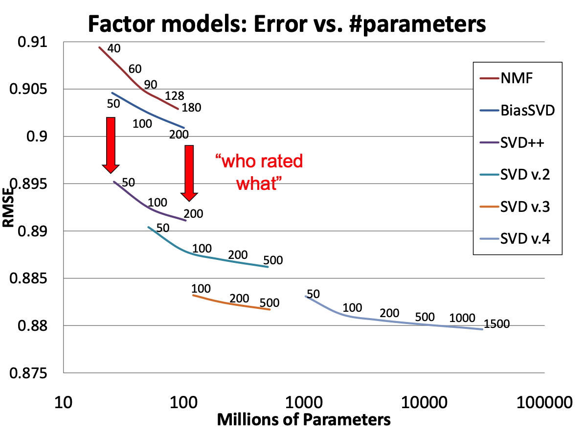
1. Adding Biases

\[ \min_{U, V} \sum_{(u, i)\in S}(r_{ui} - (\mu + \alpha_u + \beta_i + u_u^Tv_i)^2 + \lambda(\Vert U\Vert^2 + \Vert V\Vert^2 + \Vert \alpha\Vert^2 + \Vert \beta \Vert^2) \]

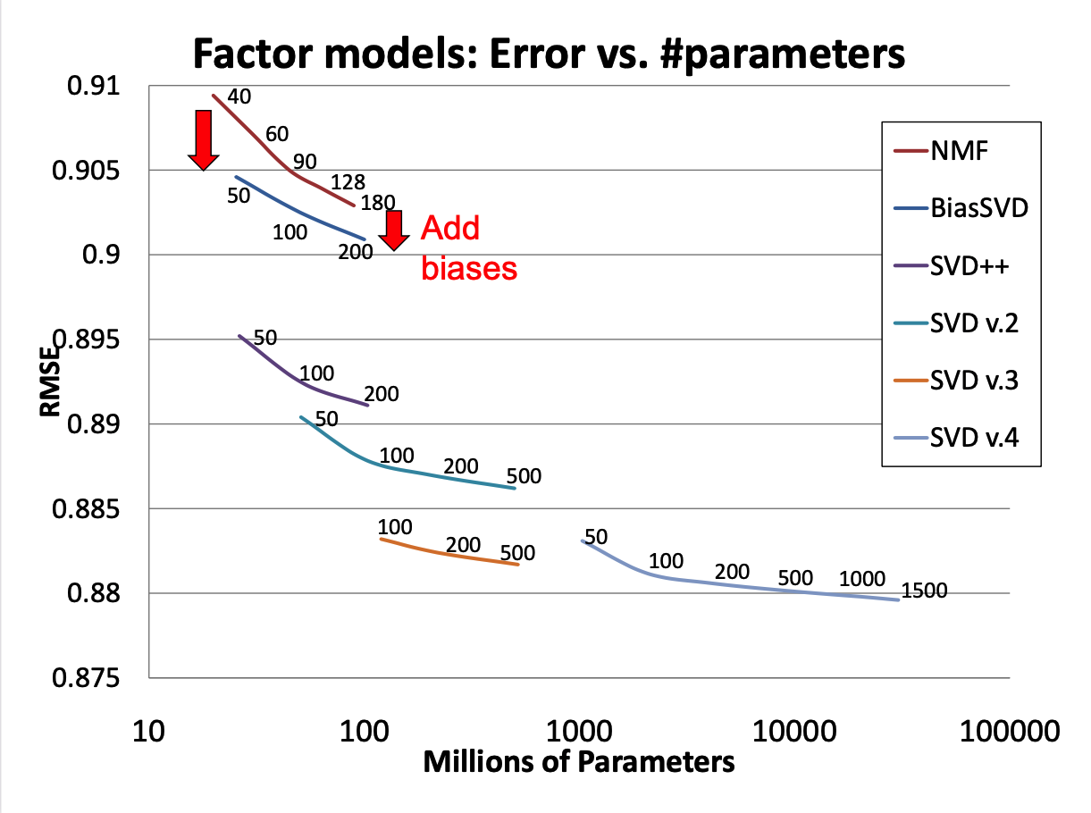
2. Who Rated What?

In reality, ratings are not provided at random.

Take note of which users rated the same movies (ala CF) and use this information.

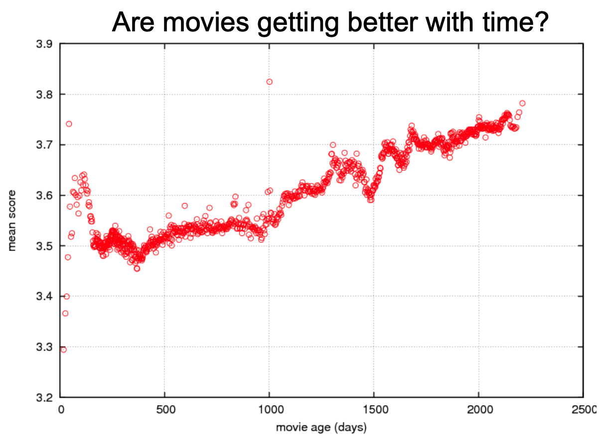
3. Ratings Change Over Time

Older movies tend to get higher ratings!

\[ \min_{U, V} \sum_{(u, i)\in S}(r_{ui} - (\mu + \alpha_u(t) + \beta_i(t) + u_u^Tv_i(t))^2 + \lambda(\Vert U\Vert^2 + \Vert V\Vert^2 + \Vert \alpha\Vert^2 + \Vert \beta \Vert^2) \]

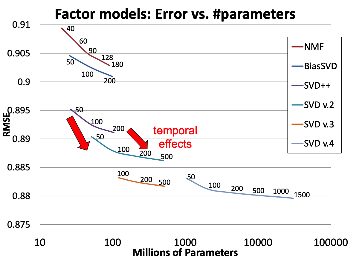
To estimate these billions of parameters, we cannot use alternating least squares or any linear algebraic method.

We need to use gradient descent (which we will cover in a future lecture).

Assessing Recommender Systems

There are a number of concerns with the widespread use of recommender systems and personalization in society.

First, recommender systems are accused of creating filter bubbles.

A filter bubble is the tendency for recommender systems to limit the variety of information presented to the user.

The concern is that a user’s past expression of interests will guide the algorithm in continuing to provide “more of the same.”

This is believed to increase polarization in society, and to reinforce confirmation bias.

Second, recommender systems in modern usage are often tuned to maximize engagement.

In other words, the objective function of the system is not to present the user’s most favored content, but rather the content that will be most likely to keep the user on the site.

The incentive to maximize engagement arises on sites that are supported by advertising revenue.

More engagement time means more revenue for the site.

However, many studies have shown that sites that strive to maximize engagement do so in large part by guiding users toward extreme content:

• content that is shocking,

• or feeds conspiracy theories,

• or presents extreme views on popular topics.

Given this tendency of modern recommender systems, for a third party to create “clickbait” content such as this, one of the easiest ways is to present false claims.

Methods for addressing these issues are being very actively studied at present.

Ways of addressing these issues can be:

• via technology

• via public policy

Note

You can read about some of the work done in my group on this topic:

• How YouTube Leads Privacy-Seeking Users Away from Reliable Information, Larissa Spinelli and Mark Crovella, Proceedings of the Workshop on Fairness in User Modeling, Adaptation, and Personalization (FairUMAP), 2020.

• Closed-Loop Opinion Formation, Larissa Spinelli and Mark Crovella Proceedings of the 9th International ACM Web Science Conference (WebSci), 2017.

• Fighting Fire with Fire: Using Antidote Data to Improve Polarization and Fairness of Recommender Systems, Bashir Rastegarpanah, Krishna P. Gummadi and Mark Crovella Proceedings of WSDM, 2019.