Show code cell source
import numpy as np
import scipy as sp
import matplotlib.pyplot as plt
import pandas as pd
import seaborn as sns
%matplotlib inline
Gaussian Mixture Models#
From Hard to Soft Clustering#
So far, we have seen how to cluster objects using \(k\)-means:
start with an initial set of cluster centers,
assign each object to its closest cluster center, and
recompute the centers of the new clusters.
Repeat 2 \(\rightarrow\) 3 until convergence.
Note that in \(k\)-means, every object is assigned to a single cluster.
This is called hard assignment.
However, there may be cases were we either cannot use hard assignments or we do not want to do it!
In particular, we may believe that the best description of the data is a set of overlapping clusters.
For example:
Imagine that we believe society consists of just two kinds of individuals: poor, or rich.
Let’s think about how we might model society as a mixture of poor and rich, when viewed in terms of age.
Say we sample 20,000 rich individuals, and 20,000 poor individuals, and get the following histograms:
Show code cell source
# original inspiration for this example from
# https://www.cs.cmu.edu/~./awm/tutorials/gmm14.pdf
from scipy.stats import multivariate_normal
np.random.seed(4)
df = pd.DataFrame(multivariate_normal.rvs(mean = np.array([37, 45]), cov = np.diag([196, 121]), size = 20000),
                   columns = ['poor', 'rich'])
df.hist(bins = range(80), sharex = True);
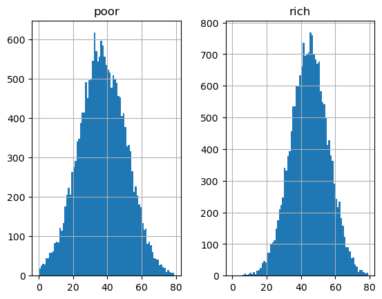
We find that ages of the poor set have mean 37 with standard deviation 14,
while the ages of the rich set have mean 45 with standard deviation 11.
Show code cell source
from scipy.stats import norm
plt.figure()
x = np.linspace(norm.ppf(0.001, loc = 37, scale = 14), norm.ppf(0.999, loc = 37, scale = 14), 100)
plt.plot(x, norm.pdf(x, loc = 37, scale = 14),'b-', lw = 5, alpha = 0.6, label = 'poor')
x = np.linspace(norm.ppf(0.001, loc = 45, scale = 11), norm.ppf(0.999, loc = 45, scale = 11), 100)
plt.plot(x, norm.pdf(x, loc = 45, scale = 11),'g-', lw = 5, alpha = 0.6, label = 'rich')
plt.xlim([15, 70])
plt.xlabel('Age', size=14)
plt.legend(loc = 'best')
plt.title('Age Distributions')
plt.ylabel(r'$p(x)$', size=14);
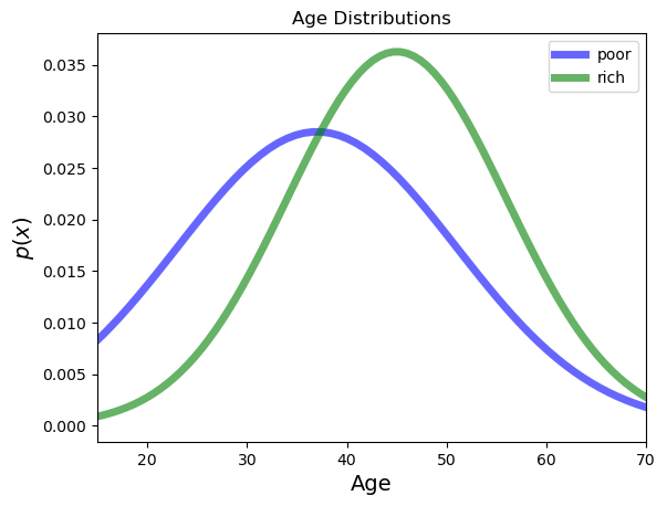
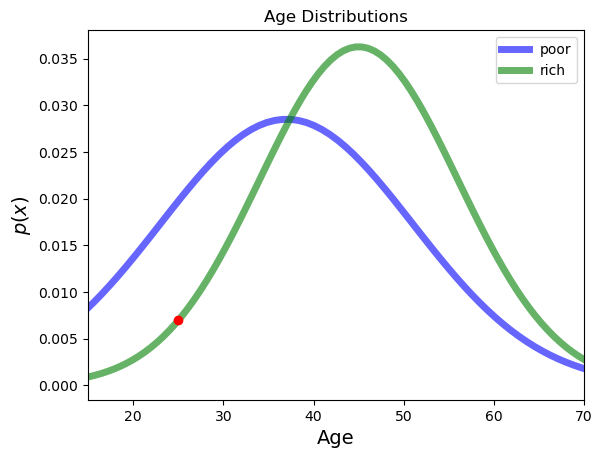
Clearly, viewed along the age dimension, there are two clusters that overlap.
Furthermore, given some particular individual at a given age, say 25, we cannot say for sure which cluster they belong to.
Rather, we will use probability to quantify our uncertainty about the cluster that any single individual belongs to.
Thus, we could say that a given individual (“John Smith”, age 25) belongs to the rich cluster with some probability, and the poor cluster with some different probability.
Naturally we expect the probabilities for John Smith to sum up to 1.
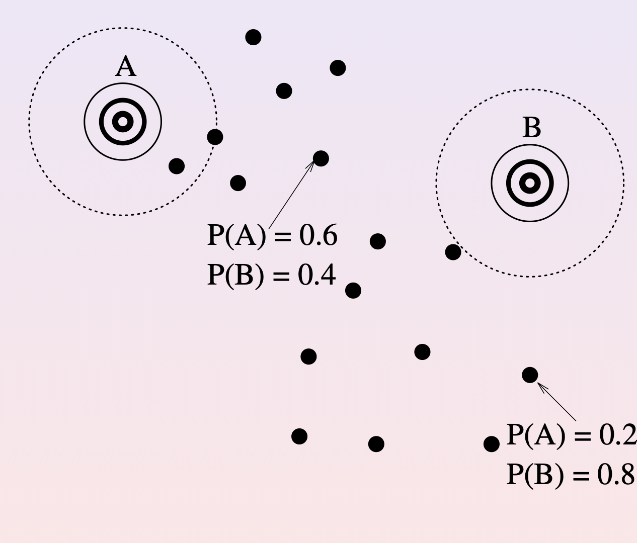
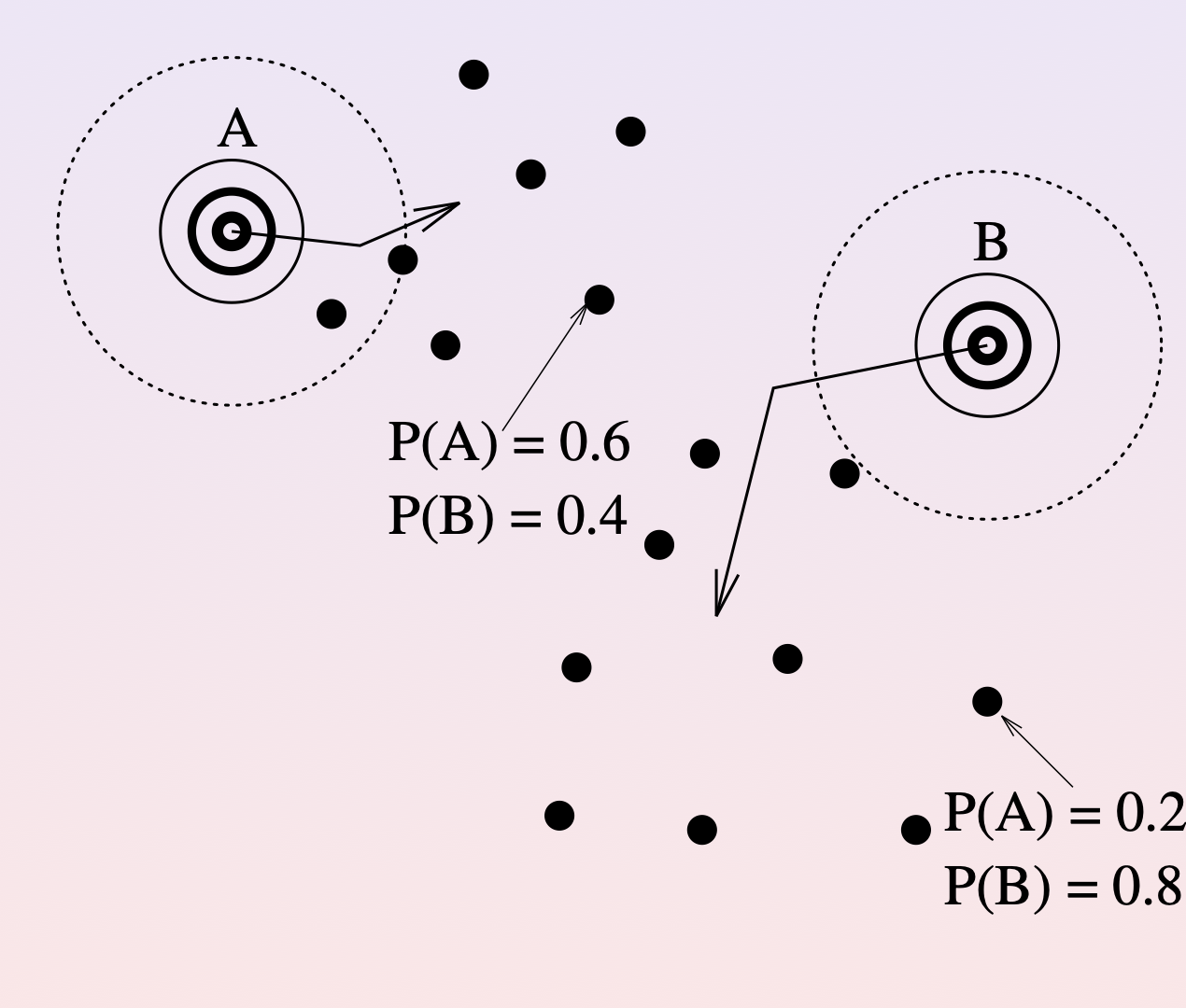
This is called soft assignment, and a clustering using this principle is called soft clustering.
More formally, we say that an object can belong to each particular cluster with some probability, such that the sum of the probabilities adds up to 1 for each object.
For example, assuming that we have two clusters \(C_1\) and \(C_2\), we can have that an object \(x_1\) belongs to \(C_1\) with probability \(0.3\) and to \(C_2\) with probability \(0.7\).
Note that the distribution over \(C_1\) and \(C_2\) only refers to object \(x_1\).
Thus, it is a conditional probability:
And to return to our previous example:
Mixtures of Gaussians#
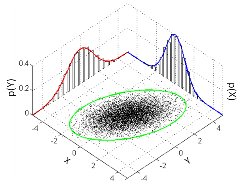
We’re going to consider a particular model for each cluster: the Gaussian (or Normal) distribution.
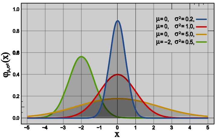
By Inductiveload - self-made, Mathematica, Inkscape, Public Domain, https://commons.wikimedia.org/w/index.php?curid=3817954
You can see that, for example, this is a reasonable model for the distribution of ages in each of the two population groups (rich and poor).
In the case of the population example, we have a single feature: age.
How do we use a Gaussian when we have multiple features?
The answer is that we use a multivariate Gaussian.
By Bscan - Own work, CC0, https://commons.wikimedia.org/w/index.php?curid=25235145
Now each point is a vector in \(n\) dimensions: \(\mathbf{x} = (x_1, \dots, x_n)^T\).
As a reminder, the multivariate Gaussian has a pdf (density) function of:
Recall also that the shape of a multivariate Gaussian – the direction of its axes and the width along each axis – is determined by the covariance matrix \(\Sigma\).
The covariance matrix is the multidimensional analog of the variance. It determines the extent to which vector components are correlated.
For example, let’s say we are looking to classify cars based on their model year and miles per gallon (mpg).
To illustrate a particular model, let us consider the properties of cars produced in the US, Europe, and Asia.
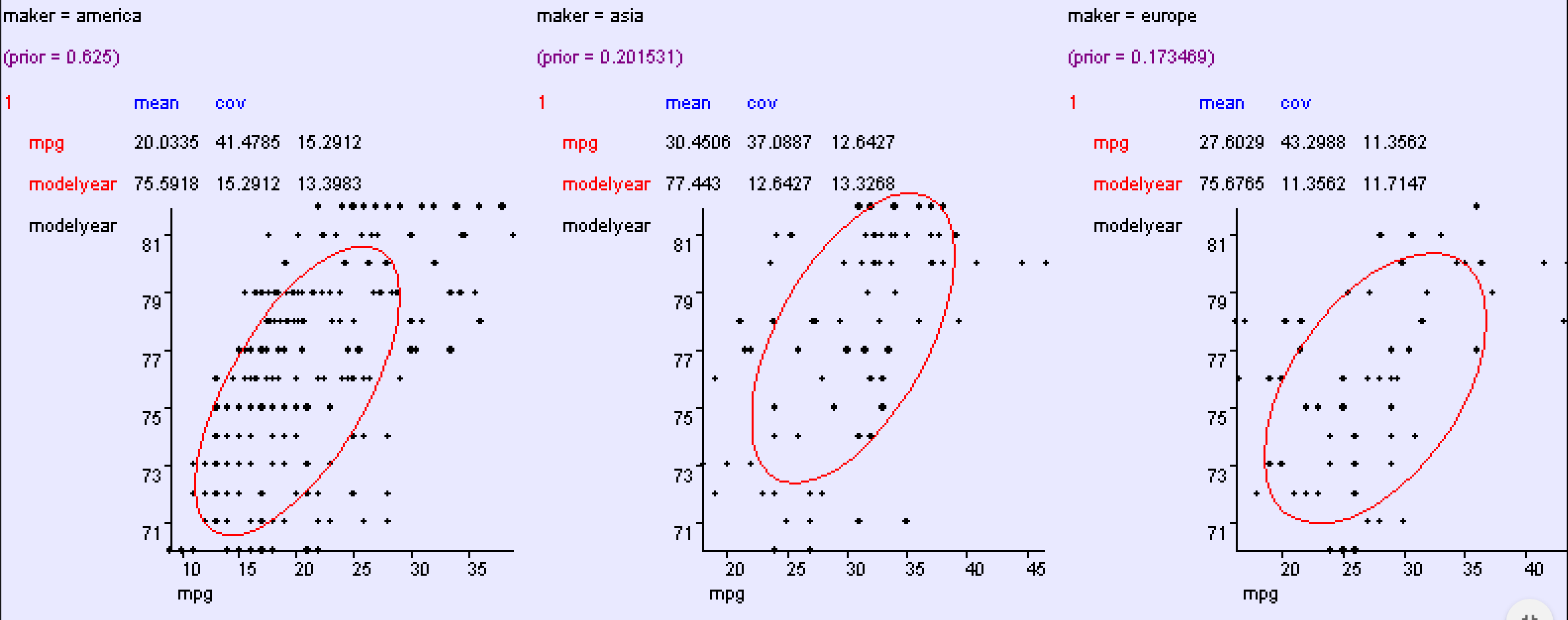
It seems that the data can be described (roughly) as a mixture of three multivariate Gaussian distributions.
The general situation is that we assume the data was generated according to a collection of arbitrary Gaussian distributions.
This is called a Gaussian Mixture Model.
Aka a “GMM”.
 Ellipsoid Representation
 Density
A Gaussian Mixture Model is defined by:
Where \(w_i\) is the prior probability (weight) of the \(i\)th Gaussian, such that
Intuitively, \(w_i\) tells us “what fraction of the data comes from Gaussian \(i\).”
Then the probability density at any point \(x\) is given by:
Learning the Parameters of a GMM#
This model is all very well, but how do we learn the parameters of such a model, given some data?
That is, assume we are told there are \(k\) clusters.
For each \(i\) in \(1, \dots, k\), how do we estimate the
cluster probability \(w_i\),
cluster mean \(\mu_i\), and
cluster covariance \(\Sigma_i\)?
There are a variety of ways of finding the best \((w_i, \mu_i, \Sigma_i)\;\;\;i = 1,\dots,k\).
We will consider the most popular method: Expectation Maximization (EM).
This is another famous algorithm, in the same “super-algorithm” league as \(k\)-means.
EM is formulated using a probabilistic model for data. It can solve a problem like:
Given a set of data points and a parameter \(k\), find the \((w_i, \mu_i, \Sigma_i)\;\;i = 1,\dots,k\) that maximizes the likelihood of the data assuming a GMM with those parameters.
(It can also solve lots of other problems involving maximizing likelihood of data under a model.)
However, note that problems of this type are often NP-hard.
EM only guarantees that it will find a local optimum of the objective function.
Probabilities We Will Use#
At a high level, EM for the GMM problem has strong similarities to \(k\)-means.
However, there are two main differences:
The \(k\)-means problem posits a hard assignment of objects to clusters, while GMM uses soft assignment.
The parameters of the soft assignment are chosed based on a probability model for the data.
Let’s start by reviewing the situation probabilistically.
Assume a set data points \(x_1, x_2,\ldots,x_n\) in a \(d\) dimensional space.
Also assume a set of \(k\) clusters \(C_1, C_2, \ldots, C_k\). Each cluster is assumed to follow a Gaussian distribution:
We will be working with conditional probabilities.
First,
\(P(x_i\,|\,C_j)\) is the probability of seeing data point \(x_i\) when sampling from cluster \(C_j\).
That is, it is the value of a Gaussian pdf at the point \(x_i\), for a Gaussian with parameters \(({\mathbf \mu_j},{\mathbf \Sigma_j})\).
Clearly, if I give you the cluster parameters, it is a straightforward thing to compute this conditional probability.
In our example: \(P(\text{age 25}\,|\,\text{rich})\)
Show code cell source
plt.figure()
x = np.linspace(norm.ppf(0.001, loc = 37, scale = 14), norm.ppf(0.999, loc = 37, scale = 14), 100)
plt.plot(x, norm.pdf(x, loc = 37, scale = 14),'b-', lw = 5, alpha = 0.6, label = 'poor')
x = np.linspace(norm.ppf(0.001, loc = 45, scale = 11), norm.ppf(0.999, loc = 45, scale = 11), 100)
plt.plot(x, norm.pdf(x, loc = 45, scale = 11),'g-', lw = 5, alpha = 0.6, label = 'rich')
plt.plot(25, norm.pdf(25, loc = 45, scale = 11), 'ro')
plt.xlim([15, 70])
plt.xlabel('Age', size=14)
plt.legend(loc = 'best')
plt.title('Age Distributions')
plt.ylabel(r'$p(x)$', size=14);
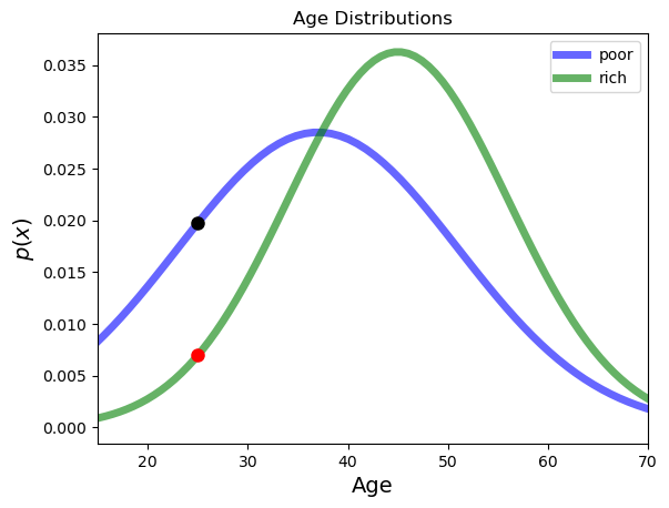
We will also work with \(P(C_j\,|\,x_i)\).
This is the probability that a data point at \(x_i\) was drawn from cluster \(C_j\).
That is, the data point could have been drawn from any of the \(k\) clusters – what is the probability it was drawn from \(C_j\) in particular?
In our example: \(P(\text{rich}\,|\,\text{age 25})\)
How can we compute \(P(C_j\,|\,x_i)\)?
Note that the reverse conditional probability is easy to compute – so this is a job for Bayes’ Rule!
Show code cell source
plt.figure()
x = np.linspace(norm.ppf(0.001, loc = 37, scale = 14), norm.ppf(0.999, loc = 37, scale = 14), 100)
plt.plot(x, norm.pdf(x, loc = 37, scale = 14),'b-', lw = 5, alpha = 0.6, label = 'poor')
plt.plot(25, norm.pdf(25, loc = 37, scale = 14), 'ko', markersize = 8)
x = np.linspace(norm.ppf(0.001, loc = 45, scale = 11), norm.ppf(0.999, loc = 45, scale = 11), 100)
plt.plot(x, norm.pdf(x, loc = 45, scale = 11),'g-', lw = 5, alpha = 0.6, label = 'rich')
plt.plot(25, norm.pdf(25, loc = 45, scale = 11), 'ro', markersize = 8)
plt.xlim([15, 70])
plt.xlabel('Age', size=14)
plt.legend(loc = 'best')
plt.title('Age Distributions')
plt.ylabel(r'$p(x)$', size=14);
Finally, we will also need to estimate the parameters of each Gaussian, given some data.
This is also an easy problem.
For example, the best estimate for the mean of a Gaussian, given some data, is the average of the data points.
Likewise, there is a simple formula for the covariance.
These are called Maximum Likelihood Estimates (MLE) of the parameters.
Often we use \(\mathbf \theta\) to denote “all the parameters of the model.”
In this case \(\mathbf \theta_i = (w_i, {\mathbf \mu_i},{\mathbf \Sigma_i})\).
Expectation Maximization for GMM – The Algorithm#
OK, now we have all the necessary pieces. Here is the algorithm.
Initialization:
Start with an initial set of clusters \(C_1^1, C_2^1, \ldots, C_k^1\) and the initial probabilities that a random point belongs to each cluster \(P(C_1), P(C_2), \ldots, P(C_k)\).
The result will be sensitive to this choice, so a good (and fast) initialization procedure is \(k\)-means.
Step 1 (Expectation): For each point \(x_i\), compute the probability that it belongs to each cluster \(C_j\):
(Thank you, Rev. Bayes!)
This is called the posterior probability of \(C_j\) given \(x_i\).
We know how to compute everything on the right.
Note that: \(P(x_i) = \sum_{j=1}^k P(x_i\,|\,C_j)\,P(C_j)\)
Step 2 (Maximization): Using the cluster membership probabilities computed in the previous step, compute new clusters (parameters) and cluster probabilities.
This is easy, using maximum likelihood estimates of the parameters \(\theta\).
Likewise, compute new parameters for the clusters \(C_1, C_2, \ldots, C_n\) using MLE.
Repeat Steps 1 and 2 until stabilization.
Let’s pause for a minute and compare GMM/EM with \(k\)-means.
GMM/EM:
Initialize randomly or using some rule
Compute the probability that each point belongs in each cluster
Update the clusters (weights, means and variances).
Repeat 2-3 until convergence.
\(k\)-means:
Initialize randomly or using some rule
Assign each point to a single cluster
Update the clusters (means).
Repeat 2-3 until convergence.
From a practical standpoint, the main difference is that in GMM, data points do not belong to a single cluster, but have some probability of belonging to each cluster.
In other words, GMM uses soft assignment.
For that reason, GMM is also sometimes called soft \(k\)-means.
However, there is also an important conceptual difference.
The GMM starts by making an explicit assumption about how the data were generated.
It says: “the data came from a collection of multivariate Gaussians.”
Note that we made no such assumption when we came up with the \(k\)-means problem. In that case, we simply defined an objective function and declared that it was a good one.
Nonetheless, it appears that we were making a sort of Gaussian assumption when we formulated the \(k\)-means objective function. However, we didn’t explicitly state it.
The point is that because the GMM makes its assumptions explicit, we can
examine them and think about whether they are valid
replace them with different assumptions if we wish
This sort of assumption is called a “prior” on the data.
Philosophically, exposing this assumption is the heart of Bayesian statistics.
For example, it is perfectly possible to replace the Gaussian assumption with some other probility distribution. As long as we can estimate the parameters of such distributions from data (eg, have MLEs), we can use EM in that case as well.
Instantiating EM with the Gaussian Model#
If we model each cluster as a multi-dimensional Gaussian, then we can instatiate every part of the algorithm.
This is the GMM (Gaussian Mixture Model) algorithm implemented in sklearn.mixture module.
In that case \(C_i\) is represented by \((\mu_i, \Sigma_i)\) and in EM Step 1 we compute:
In EM Step 2, we estimate the parameters of the Gaussian using the appropriate MLEs:
and
A final statement about EM generally. EM is a versatile algorithm that can be used in many other settings. What is the main idea behind it?
Notice that the problem definition only required that we find the clusters, \(C_i\), meaning that we were to find the \((\mu_i, \Sigma_i)\).
However, the EM algorithm posited that we should find as well the \(P(C_j|x_i)\), that is, the probability that each point is a member of each cluster.
This is the true heart of what EM does.
The idea is called “data augmentation.”
By adding parameters to the problem, it actually finds a way to make the problem solvable!
These parameters don’t show up in the solution. They are sometimes called “hidden parameters.”
So the basic strategy for using EM is: think up some additional information which, if you had it, would make the problem solvable.
Figure out how to estimate the additional information from a solved problem, and put the two steps into a loop.
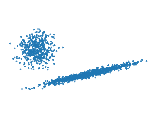
Here is an example using GMM.
We’re going to create two clusters, one spherical, and one highly skewed.
# Number of samples of larger component
n_samples = 1000

# C is a transfomation that will make a heavily skewed 2-D Gaussian
C = np.array([[0.1, -0.1], [1.7, .4]])

print(f'The covariance matrix of our skewed cluster will be:\n {C.T@C}')
The covariance matrix of our skewed cluster will be:
 [[2.9  0.67]
 [0.67 0.17]]
# make the sample deterministic
np.random.seed(0)

# now we construct a data matrix that has n_samples from the skewed distribution,
# and n_samples/2 from a symmetric distribution offset to position (-4, 2)
X = np.r_[(np.random.randn(n_samples, 2) @ C),
          .7 * np.random.randn(n_samples//2, 2) + np.array([-4, 2])]
Show code cell source
plt.scatter(X[:, 0], X[:, 1], s = 10, alpha = 0.8)
plt.axis('equal')
plt.axis('off');
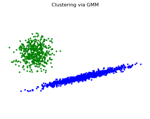
# Fit a mixture of Gaussians with EM using two components
import sklearn.mixture
gmm = sklearn.mixture.GaussianMixture(n_components=2,
                                      covariance_type='full',
                                      init_params = 'kmeans')
y_pred = gmm.fit_predict(X)
Show code cell source
colors = ['bg'[p] for p in y_pred]
plt.title('Clustering via GMM')
plt.axis('off')
plt.axis('equal')
plt.scatter(X[:, 0], X[:, 1], color = colors, s = 10, alpha = 0.8);
Show code cell source
for clus in range(2):
    print(f'Cluster {clus}:')
    print(f' weight: {gmm.weights_[clus]:0.3f}')
    print(f' mean: {gmm.means_[clus]}')
    print(f' cov: \n{gmm.covariances_[clus]}\n')
Cluster 0:
 weight: 0.667
 mean: [-0.01895709 -0.00177815]
 cov:
[[2.79024354 0.64760422]
 [0.64760422 0.16476598]]

Cluster 1:
 weight: 0.333
 mean: [-4.05403279  1.9822596 ]
 cov:
[[0.464702   0.02385764]
 [0.02385764 0.42700883]]
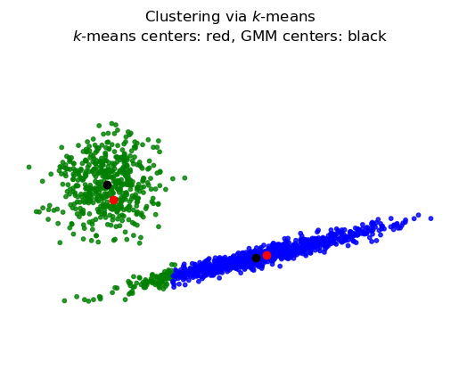
Show code cell source
import sklearn.cluster
kmeans = sklearn.cluster.KMeans(init = 'k-means++', n_clusters = 2, n_init = 100)
y_pred_kmeans = kmeans.fit_predict(X)
colors = ['bg'[p] for p in y_pred_kmeans]
plt.title('Clustering via $k$-means\n$k$-means centers: red, GMM centers: black')
plt.axis('off')
plt.axis('equal')
plt.scatter(X[:, 0], X[:, 1], color = colors, s = 10, alpha = 0.8)
plt.plot(kmeans.cluster_centers_[:,0], kmeans.cluster_centers_[:,1], 'ro')
plt.plot(gmm.means_[:,0], gmm.means_[:,1], 'ko');
Show code cell source
for clus in range(2):
    print(f'Cluster {clus}:')
    print(f' center: {kmeans.cluster_centers_[clus]}\n')
Cluster 0:
 center: [0.28341737 0.06741478]

Cluster 1:
 center: [-3.88381453  1.56532945]
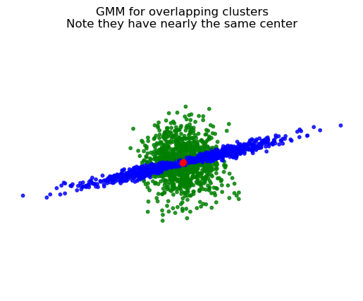
Now, let’s construct overlapping clusters. What will happen?
X = np.r_[np.random.randn(n_samples, 2) @ C,
          0.7 * np.random.randn(n_samples, 2) ]
gmm = sklearn.mixture.GaussianMixture(n_components=2, covariance_type='full')
y_pred_over = gmm.fit_predict(X)
Show code cell source
colors = ['bgrky'[p] for p in y_pred_over]
plt.title('GMM for overlapping clusters\nNote they have nearly the same center')
plt.scatter(X[:, 0], X[:, 1], color = colors, s = 10, alpha = 0.8)
plt.axis('equal')
plt.axis('off')
plt.plot(gmm.means_[:,0], gmm.means_[:,1], 'ro');
Show code cell source
for clus in range(2):
    print(f'Cluster {clus}:')
    print(f' weight: {gmm.weights_[clus]:0.3f}')
    print(f' mean: {gmm.means_[clus]}\n')
    # print(f' cov: \n{gmm.covariances_[clus]}\n')
Cluster 0:
 weight: 0.507
 mean: [0.00881243 0.00217253]

Cluster 1:
 weight: 0.493
 mean: [ 0.00346227 -0.00250677]
How many parameters are estimated?#
Most of the parameters in the model are contained in the covariance matrices.
In the most general case, for \(k\) clusters of points in \(n\) dimensions, there are \(k\) covariance matrices each of size \(n \times n\).
So we need \(kn^2\) parameters to specify this model.
It can happen that you may not have enough data to estimate so many parameters.
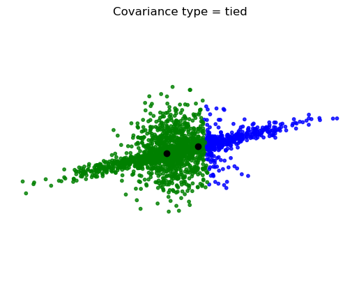
Also, it can happen that you believe that clusters should have some constraints on their shapes.
Here is where the GMM assumptions become really useful.
Let’s say you believe all the clusters should have the same shape, but the shape can be arbitrary.
Then you only need to estimate one covariance matrix - just \(n^2\) parameters.
This is specified by the GMM parameter covariance_type='tied'.
X = np.r_[np.dot(np.random.randn(n_samples, 2), C),
          0.7 * np.random.randn(n_samples, 2) ]
gmm = sklearn.mixture.GaussianMixture(n_components=2, covariance_type='tied')
y_pred = gmm.fit_predict(X)
Show code cell source
colors = ['bgrky'[p] for p in y_pred]
plt.scatter(X[:, 0], X[:, 1], color=colors, s=10, alpha=0.8)
plt.title('Covariance type = tied')
plt.axis('equal')
plt.axis('off')
plt.plot(gmm.means_[:,0],gmm.means_[:,1], 'ok');
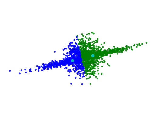
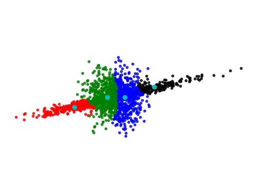
Perhaps you believe in even more restricted shapes: all clusters should have their axes aligned with the coordinate axes.
That is, clusters are not skewed.
Then you only need to estimate the diagonals of the covariance matrices - just \(kn\) parameters.
This is specified by the GMM parameter covariance_type='diag'.
X = np.r_[np.dot(np.random.randn(n_samples, 2), C),
          0.7 * np.random.randn(n_samples, 2)]
gmm = sklearn.mixture.GaussianMixture(n_components=4, covariance_type='diag')
y_pred = gmm.fit_predict(X)
Show code cell source
colors = ['bgrky'[p] for p in y_pred]
plt.scatter(X[:, 0], X[:, 1], color = colors, s = 10, alpha = 0.8)
plt.axis('equal')
plt.axis('off')
plt.plot(gmm.means_[:,0], gmm.means_[:,1], 'oc');
Finally, if you believe that all clusters should be round, then you only need to estimate the \(k\) variances.
This is specified by the GMM parameter covariance_type='spherical'.
X = np.r_[np.dot(np.random.randn(n_samples, 2), C),
          0.7 * np.random.randn(n_samples, 2)]
gmm = sklearn.mixture.GaussianMixture(n_components=2, covariance_type='spherical')
y_pred = gmm.fit_predict(X)
Show code cell source
colors = ['bgrky'[p] for p in y_pred]
plt.scatter(X[:, 0], X[:, 1], color = colors, s = 10, alpha = 0.8)
plt.axis('equal')
plt.axis('off')
plt.plot(gmm.means_[:,0], gmm.means_[:,1], 'oc');