Essential Tools: Pandas

Essential Tools: Pandas#

Pandas is the Python Data Analysis Library.

Pandas is an extremely versatile tool for manipulating datasets.

It also produces high quality plots with matplotlib, and integrates nicely with other libraries that expect NumPy arrays.

Use of Pandas is a data science best practice.

The most important tool provided by Pandas is the data frame.

A data frame is a table in which each row and column is given a label.

Pandas DataFrames are documented at:

http://pandas.pydata.org/pandas-docs/dev/generated/pandas.DataFrame.html

Get in the habit: whenever you load data, place it into a dataframe as your first step.

Getting started#

import pandas as pd
import pandas_datareader.data as web
from pandas import Series, DataFrame

import matplotlib.pyplot as plt
import seaborn as sns

from datetime import datetime

#pd.__version__

%matplotlib inline

Fetching, storing and retrieving your data#

For demonstration purposes, we’ll use a utility library that fetches data from standard online sources, such as Yahoo! Finance.

import yfinance as yf

yahoo_stocks = pd.DataFrame(yf.download('YELP',start='2015-01-01',end='2015-12-31', progress = False))

yahoo_stocks.head()

	Open	High	Low	Close	Adj Close	Volume
Date
2015-01-02	55.459999	55.599998	54.240002	55.150002	55.150002	1664500
2015-01-05	54.540001	54.950001	52.330002	52.529999	52.529999	2023000
2015-01-06	52.549999	53.930000	50.750000	52.439999	52.439999	3762800
2015-01-07	53.320000	53.750000	51.759998	52.209999	52.209999	1548200
2015-01-08	52.590000	54.139999	51.759998	53.830002	53.830002	2015300

This is a typical example of a dataframe.

Notice how each row has a label and each column has a label.

A dataframe is an object that has many methods associated with it, to do all sorts of useful things.

Here is a simple method: .info()

yahoo_stocks.info()

<class 'pandas.core.frame.DataFrame'>
DatetimeIndex: 251 entries, 2015-01-02 to 2015-12-30
Data columns (total 6 columns):
 #   Column     Non-Null Count  Dtype  
---  ------     --------------  -----  
 0   Open       251 non-null    float64
 1   High       251 non-null    float64
 2   Low        251 non-null    float64
 3   Close      251 non-null    float64
 4   Adj Close  251 non-null    float64
 5   Volume     251 non-null    int64  
dtypes: float64(5), int64(1)
memory usage: 13.7 KB

Reading to/from a `.csv` file#

Continuing to explore methods, let’s write the dataframe out to a .csv file:

yahoo_stocks.to_csv('yahoo_data.csv')

!head yahoo_data.csv

Date,Open,High,Low,Close,Adj Close,Volume
2015-01-02,55.459999084472656,55.599998474121094,54.2400016784668,55.150001525878906,55.150001525878906,1664500
2015-01-05,54.540000915527344,54.95000076293945,52.33000183105469,52.529998779296875,52.529998779296875,2023000
2015-01-06,52.54999923706055,53.93000030517578,50.75,52.439998626708984,52.439998626708984,3762800
2015-01-07,53.31999969482422,53.75,51.7599983215332,52.209999084472656,52.209999084472656,1548200
2015-01-08,52.59000015258789,54.13999938964844,51.7599983215332,53.83000183105469,53.83000183105469,2015300
2015-01-09,55.959999084472656,56.9900016784668,54.720001220703125,56.06999969482422,56.06999969482422,6224200
2015-01-12,56.0,56.060001373291016,53.43000030517578,54.02000045776367,54.02000045776367,2407700
2015-01-13,54.470001220703125,54.79999923706055,52.52000045776367,53.18000030517578,53.18000030517578,1958400
2015-01-14,52.79999923706055,53.68000030517578,51.459999084472656,52.20000076293945,52.20000076293945,1854600

And of course we can likewise read a .csv file into a dataframe. This is probably the most common way you will get data into Pandas.

df = pd.read_csv('yahoo_data.csv')
df.head()

	Date	Open	High	Low	Close	Adj Close	Volume
0	2015-01-02	55.459999	55.599998	54.240002	55.150002	55.150002	1664500
1	2015-01-05	54.540001	54.950001	52.330002	52.529999	52.529999	2023000
2	2015-01-06	52.549999	53.930000	50.750000	52.439999	52.439999	3762800
3	2015-01-07	53.320000	53.750000	51.759998	52.209999	52.209999	1548200
4	2015-01-08	52.590000	54.139999	51.759998	53.830002	53.830002	2015300

Working with data columns#

In general, we’ll usually organize things so that rows in the dataframe are items and columns are features.

df.columns

Index(['Date', 'Open', 'High', 'Low', 'Close', 'Adj Close', 'Volume'], dtype='object')

Pandas allows you to use standard python indexing to refer to columns (eg features) in your dataframe:

df['Open']

    55.459999
    54.540001
    52.549999
    53.320000
    52.590000
         ...    
  27.950001
  28.270000
  28.120001
  27.950001
  28.580000
Name: Open, Length: 251, dtype: float64

Pandas also allows you to use a syntax like an object attribute to refer to a column.

But note that the column name cannot include a space in this case.

df.Open

    55.459999
    54.540001
    52.549999
    53.320000
    52.590000
         ...    
  27.950001
  28.270000
  28.120001
  27.950001
  28.580000
Name: Open, Length: 251, dtype: float64

You can select a list of columns:

df[['Open','Close']].head()

	Open	Close
0	55.459999	55.150002
1	54.540001	52.529999
2	52.549999	52.439999
3	53.320000	52.209999
4	52.590000	53.830002

Putting things together – make sure this syntax is clear to you:

df.Date.head(10)

  2015-01-02
  2015-01-05
  2015-01-06
  2015-01-07
  2015-01-08
  2015-01-09
  2015-01-12
  2015-01-13
  2015-01-14
  2015-01-15
Name: Date, dtype: object

df.Date.tail(10)

  2015-12-16
  2015-12-17
  2015-12-18
  2015-12-21
  2015-12-22
  2015-12-23
  2015-12-24
  2015-12-28
  2015-12-29
  2015-12-30
Name: Date, dtype: object

Changing column names is as simple as assigning to the .columns property.

Let’s adjust column names so that none of them include spaces:

new_column_names = [x.lower().replace(' ','_') for x in df.columns]
df.columns = new_column_names
df.info()

<class 'pandas.core.frame.DataFrame'>
RangeIndex: 251 entries, 0 to 250
Data columns (total 7 columns):
 #   Column     Non-Null Count  Dtype  
---  ------     --------------  -----  
 0   date       251 non-null    object 
 1   open       251 non-null    float64
 2   high       251 non-null    float64
 3   low        251 non-null    float64
 4   close      251 non-null    float64
 5   adj_close  251 non-null    float64
 6   volume     251 non-null    int64  
dtypes: float64(5), int64(1), object(1)
memory usage: 13.9+ KB

(Be sure you understand the list comprehension used above – it’s a common and important way to process a list in python.)

Now all columns can be accessed using the dot notation:

df.adj_close.head()

  55.150002
  52.529999
  52.439999
  52.209999
  53.830002
Name: adj_close, dtype: float64

A sampling of DataFrame methods.#

A dataframe object has many useful methods.

Familiarize yourself with dataframe methods – they are very useful.

These should be self-explanatory.

df[['high', 'low', 'open', 'close', 'volume', 'adj_close']].mean()

high         3.809084e+01
low          3.659777e+01
open         3.732426e+01
close        3.733303e+01
volume       3.501135e+06
adj_close    3.733303e+01
dtype: float64

df[['high', 'low', 'open', 'close', 'volume', 'adj_close']].std()

high         1.138931e+01
low          1.114006e+01
open         1.128846e+01
close        1.126194e+01
volume       4.152341e+06
adj_close    1.126194e+01
dtype: float64

df[['high', 'low', 'open', 'close', 'volume', 'adj_close']].median()

high         3.909000e+01
low          3.665000e+01
open         3.822000e+01
close        3.818000e+01
volume       2.356000e+06
adj_close    3.818000e+01
dtype: float64

df.open.mean()

37.3242629229785

df.high.mean()

38.09083672633684

Plotting methods#

Pandas has an extensive library of plotting functions, and they are very easy to use.

These are your “first look” functions.

(Later you will use specialized graphics packages for more sophisticated visualizations.)

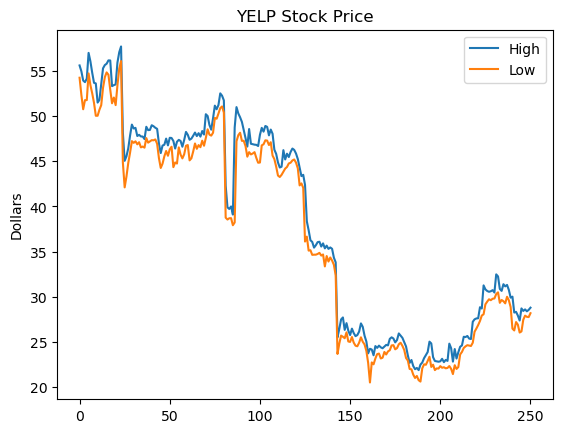
df.high.plot(label='High')
df.low.plot(label='Low')
plt.title('YELP Stock Price')
plt.ylabel('Dollars')
plt.legend(loc='best');

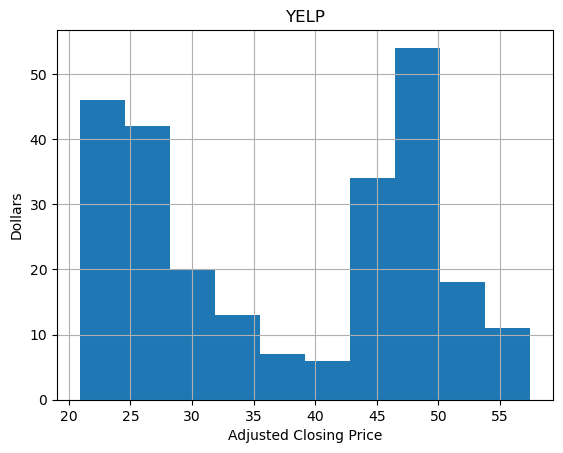
_images/32ea0100910636826e2fb2cda7ce824300ea12fd01a41762cc9da40b14859886.png

df.adj_close.hist()
plt.xlabel('Adjusted Closing Price')
plt.ylabel('Dollars')
plt.title('YELP');

_images/35ec8461fc88f64c4f89fe6a33a0b6c81592a60004774886c6962e1ede57b84b.png

Bulk Operations#

Methods like sum() and std() work on entire columns.

We can run our own functions across all values in a column (or row) using apply().

As an example, let’s go back to this plot:

df.high.plot(label='High')
df.low.plot(label='Low')
plt.title('YELP Stock Price')
plt.ylabel('Dollars')
plt.legend(loc='best');

It’s almost perfect. The only problem is the \(x\)-axis: it should show time.

To fix this, we need to make the dataframe index – that is, the row labels – into dates.

We have a problem however: the “dates” in our data are only strings. We need Pandas to understand that they are actually dates.

df.date.head()

  2015-01-02
  2015-01-05
  2015-01-06
  2015-01-07
  2015-01-08
Name: date, dtype: object

The values property of the column returns a list of values for the column. Inspecting the first value reveals that these are strings with a particular format.

first_date = df.date.values[0]
first_date

'2015-01-02'

To convert these strings to actual dates we’ll use the datetime standard python package:

datetime.strptime(first_date, "%Y-%m-%d")

datetime.datetime(2015, 1, 2, 0, 0)

And to do this for each string in the date column we will use .apply():

new_df = df.copy()
new_df.date = df.date.apply(lambda d: datetime.strptime(d, "%Y-%m-%d"))
new_df.date.head()

 2015-01-02
 2015-01-05
 2015-01-06
 2015-01-07
 2015-01-08
Name: date, dtype: datetime64[ns]

Each row in a DataFrame is associated with an index, which is a label that uniquely identifies a row.

The row indices so far have been auto-generated by pandas, and are simply integers starting from 0.

Fixing this is as easy as assigning to the index property of the DataFrame.

new_df.index = new_df.date
new_df.head()

	date	open	high	low	close	adj_close	volume
date
2015-01-02	2015-01-02	55.459999	55.599998	54.240002	55.150002	55.150002	1664500
2015-01-05	2015-01-05	54.540001	54.950001	52.330002	52.529999	52.529999	2023000
2015-01-06	2015-01-06	52.549999	53.930000	50.750000	52.439999	52.439999	3762800
2015-01-07	2015-01-07	53.320000	53.750000	51.759998	52.209999	52.209999	1548200
2015-01-08	2015-01-08	52.590000	54.139999	51.759998	53.830002	53.830002	2015300

Now that we have made an index based on a real date, we can drop the original date column.

new_df = new_df.drop(['date'],axis=1)
new_df.head()

	open	high	low	close	adj_close	volume
date
2015-01-02	55.459999	55.599998	54.240002	55.150002	55.150002	1664500
2015-01-05	54.540001	54.950001	52.330002	52.529999	52.529999	2023000
2015-01-06	52.549999	53.930000	50.750000	52.439999	52.439999	3762800
2015-01-07	53.320000	53.750000	51.759998	52.209999	52.209999	1548200
2015-01-08	52.590000	54.139999	51.759998	53.830002	53.830002	2015300

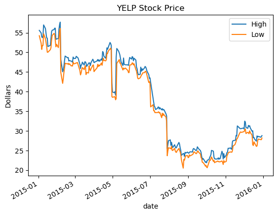
Now we can see that Pandas handles these dates quite nicely:

new_df.high.plot(label='High')
new_df.low.plot(label='Low')
plt.title('YELP Stock Price')
plt.ylabel('Dollars')
plt.legend(loc='best');

_images/a39f5c385d6e934469bd0efdc9f6a615c192668b3a0a0bc7e35945e38cf8e4e1.png

Accessing rows of the DataFrame#

So far we’ve seen how to access a column of the DataFrame. To access a row we use a different notation.

To access a row by its index value, use the .loc() method.

new_df.loc[datetime(2015,1,23,0,0)]

open         5.466000e+01
high         5.564000e+01
low          5.430000e+01
close        5.519000e+01
adj_close    5.519000e+01
volume       1.636400e+06
Name: 2015-01-23 00:00:00, dtype: float64

To access a row by its sequence number (ie, like an array index), use .iloc() (‘Integer Location’)

new_df.iloc[0,:]

open         5.546000e+01
high         5.560000e+01
low          5.424000e+01
close        5.515000e+01
adj_close    5.515000e+01
volume       1.664500e+06
Name: 2015-01-02 00:00:00, dtype: float64

To iterate over the rows, use .iterrows()

num_positive_days = 0
for idx, row in df.iterrows():
    if row.close > row.open:
        num_positive_days += 1
        
print("The total number of positive-gain days is {}.".format(num_positive_days))

The total number of positive-gain days is 125.

Filtering#

It is easy to select interesting rows from the data.

All the operations below return a new DataFrame, which itself can be treated the same way as all DataFrames we have seen so far.

tmp_high = new_df.high > 55
tmp_high.head()

date
2015-01-02     True
2015-01-05    False
2015-01-06    False
2015-01-07    False
2015-01-08    False
Name: high, dtype: bool

Summing a Boolean array is the same as counting the number of True values.

sum(tmp_high)

Now, let’s select only the rows of df1 that correspond to tmp_high

new_df[tmp_high]

	open	high	low	close	adj_close	volume
date
2015-01-02	55.459999	55.599998	54.240002	55.150002	55.150002	1664500
2015-01-09	55.959999	56.990002	54.720001	56.070000	56.070000	6224200
2015-01-12	56.000000	56.060001	53.430000	54.020000	54.020000	2407700
2015-01-22	53.869999	55.279999	53.119999	54.799999	54.799999	2295400
2015-01-23	54.660000	55.639999	54.299999	55.189999	55.189999	1636400
2015-01-26	55.119999	55.790001	54.830002	55.410000	55.410000	1450300
2015-01-27	56.060001	56.160000	54.570000	55.630001	55.630001	2410400
2015-01-28	56.150002	56.150002	52.919998	53.000000	53.000000	2013100
2015-02-03	53.830002	55.930000	53.410000	55.779999	55.779999	2885400
2015-02-04	55.529999	57.070000	55.250000	56.740002	56.740002	2498600
2015-02-05	57.599998	57.700001	56.080002	57.470001	57.470001	4657300

Putting it all together, we have the following commonly-used patterns:

positive_days = new_df[new_df.close > new_df.open]
positive_days.head()

	open	high	low	close	adj_close	volume
date
2015-01-08	52.590000	54.139999	51.759998	53.830002	53.830002	2015300
2015-01-09	55.959999	56.990002	54.720001	56.070000	56.070000	6224200
2015-01-16	50.180000	51.490002	50.029999	51.389999	51.389999	2183300
2015-01-21	51.200001	53.500000	51.200001	53.410000	53.410000	3248100
2015-01-22	53.869999	55.279999	53.119999	54.799999	54.799999	2295400

very_positive_days = new_df[(new_df.close - new_df.open) > 4]
very_positive_days.head()

	open	high	low	close	adj_close	volume
date
2015-05-07	38.220001	48.73	38.220001	47.009998	47.009998	33831600

Creating new columns#

To create a new column, simply assign values to it. Think of the columns as a dictionary:

new_df['profit'] = (new_df.open < new_df.close)
new_df.head()

	open	high	low	close	adj_close	volume	profit
date
2015-01-02	55.459999	55.599998	54.240002	55.150002	55.150002	1664500	False
2015-01-05	54.540001	54.950001	52.330002	52.529999	52.529999	2023000	False
2015-01-06	52.549999	53.930000	50.750000	52.439999	52.439999	3762800	False
2015-01-07	53.320000	53.750000	51.759998	52.209999	52.209999	1548200	False
2015-01-08	52.590000	54.139999	51.759998	53.830002	53.830002	2015300	True

Let’s give each row a gain value as a categorical variable:

for idx, row in new_df.iterrows():
    if row.open > row.close:
        new_df.loc[idx,'gain']='negative'
    elif (row.close - row.open) < 1:
        new_df.loc[idx,'gain']='small_gain'
    elif (row.close - row.open) < 6:
        new_df.loc[idx,'gain']='medium_gain'
    else:
        new_df.loc[idx,'gain']='large_gain'
new_df.head()

	open	high	low	close	adj_close	volume	profit	gain
date
2015-01-02	55.459999	55.599998	54.240002	55.150002	55.150002	1664500	False	negative
2015-01-05	54.540001	54.950001	52.330002	52.529999	52.529999	2023000	False	negative
2015-01-06	52.549999	53.930000	50.750000	52.439999	52.439999	3762800	False	negative
2015-01-07	53.320000	53.750000	51.759998	52.209999	52.209999	1548200	False	negative
2015-01-08	52.590000	54.139999	51.759998	53.830002	53.830002	2015300	True	medium_gain

Here is another, more “functional”, way to accomplish the same thing.

Define a function that classifies rows, and apply it to each row.

def namerow(row):
    if row.open > row.close:
        return 'negative'
    elif (row.close - row.open) < 1:
        return 'small_gain'
    elif (row.close - row.open) < 6:
        return 'medium_gain'
    else:
        return 'large_gain'

new_df['test_column'] = new_df.apply(namerow, axis = 1)

new_df.head()

	open	high	low	close	adj_close	volume	profit	gain	test_column
date
2015-01-02	55.459999	55.599998	54.240002	55.150002	55.150002	1664500	False	negative	negative
2015-01-05	54.540001	54.950001	52.330002	52.529999	52.529999	2023000	False	negative	negative
2015-01-06	52.549999	53.930000	50.750000	52.439999	52.439999	3762800	False	negative	negative
2015-01-07	53.320000	53.750000	51.759998	52.209999	52.209999	1548200	False	negative	negative
2015-01-08	52.590000	54.139999	51.759998	53.830002	53.830002	2015300	True	medium_gain	medium_gain

OK, point made, let’s get rid of that extraneous test_column:

new_df.drop('test_column', axis = 1)

	open	high	low	close	adj_close	volume	profit	gain
date
2015-01-02	55.459999	55.599998	54.240002	55.150002	55.150002	1664500	False	negative
2015-01-05	54.540001	54.950001	52.330002	52.529999	52.529999	2023000	False	negative
2015-01-06	52.549999	53.930000	50.750000	52.439999	52.439999	3762800	False	negative
2015-01-07	53.320000	53.750000	51.759998	52.209999	52.209999	1548200	False	negative
2015-01-08	52.590000	54.139999	51.759998	53.830002	53.830002	2015300	True	medium_gain
...	...	...	...	...	...	...	...	...
2015-12-23	27.950001	28.420000	27.440001	28.150000	28.150000	1001000	True	small_gain
2015-12-24	28.270000	28.590000	27.900000	28.400000	28.400000	587400	True	small_gain
2015-12-28	28.120001	28.379999	27.770000	27.879999	27.879999	1004500	False	negative
2015-12-29	27.950001	28.540001	27.740000	28.480000	28.480000	1103900	True	small_gain
2015-12-30	28.580000	28.780001	28.170000	28.250000	28.250000	1068000	False	negative

251 rows × 8 columns

Grouping#

An extremely powerful DataFrame method is groupby().

This is entirely analagous to GROUP BY in SQL.

It will group the rows of a DataFrame by the values in one (or more) columns, and let you iterate through each group.

Here we will look at the average gain among the categories of gains (negative, small, medium and large) we defined above and stored in column gain.

gain_groups = new_df.groupby('gain')

Essentially, gain_groups behaves like a dictionary:

the keys are the unique values found in the gain column, and
the values are DataFrames that contain only the rows having the corresponding unique values.

for gain, gain_data in gain_groups:
    print(gain)
    print(gain_data.head())
    print('=============================')

large_gain
                 open   high        low      close  adj_close    volume  \
date                                                                      
2015-05-07  38.220001  48.73  38.220001  47.009998  47.009998  33831600   

            profit        gain test_column  
date                                        
2015-05-07    True  large_gain  large_gain  
=============================
medium_gain
                 open       high        low      close  adj_close   volume  \
date                                                                         
2015-01-08  52.590000  54.139999  51.759998  53.830002  53.830002  2015300   
2015-01-16  50.180000  51.490002  50.029999  51.389999  51.389999  2183300   
2015-01-21  51.200001  53.500000  51.200001  53.410000  53.410000  3248100   
2015-02-03  53.830002  55.930000  53.410000  55.779999  55.779999  2885400   
2015-02-04  55.529999  57.070000  55.250000  56.740002  56.740002  2498600   

            profit         gain  test_column  
date                                          
2015-01-08    True  medium_gain  medium_gain  
2015-01-16    True  medium_gain  medium_gain  
2015-01-21    True  medium_gain  medium_gain  
2015-02-03    True  medium_gain  medium_gain  
2015-02-04    True  medium_gain  medium_gain  
=============================
negative
                 open       high        low      close  adj_close   volume  \
date                                                                         
2015-01-02  55.459999  55.599998  54.240002  55.150002  55.150002  1664500   
2015-01-05  54.540001  54.950001  52.330002  52.529999  52.529999  2023000   
2015-01-06  52.549999  53.930000  50.750000  52.439999  52.439999  3762800   
2015-01-07  53.320000  53.750000  51.759998  52.209999  52.209999  1548200   
2015-01-12  56.000000  56.060001  53.430000  54.020000  54.020000  2407700   

            profit      gain test_column  
date                                      
2015-01-02   False  negative    negative  
2015-01-05   False  negative    negative  
2015-01-06   False  negative    negative  
2015-01-07   False  negative    negative  
2015-01-12   False  negative    negative  
=============================
small_gain
                 open       high        low      close  adj_close   volume  \
date                                                                         
2015-01-09  55.959999  56.990002  54.720001  56.070000  56.070000  6224200   
2015-01-22  53.869999  55.279999  53.119999  54.799999  54.799999  2295400   
2015-01-23  54.660000  55.639999  54.299999  55.189999  55.189999  1636400   
2015-01-26  55.119999  55.790001  54.830002  55.410000  55.410000  1450300   
2015-01-29  52.849998  53.310001  51.410000  52.930000  52.930000  1844100   

            profit        gain test_column  
date                                        
2015-01-09    True  small_gain  small_gain  
2015-01-22    True  small_gain  small_gain  
2015-01-23    True  small_gain  small_gain  
2015-01-26    True  small_gain  small_gain  
2015-01-29    True  small_gain  small_gain  
=============================

for gain, gain_data in new_df.groupby("gain"):
    print('The average closing value for the {} group is {}'.format(gain,
                                                           gain_data.close.mean()))

The average closing value for the large_gain group is 47.0099983215332
The average closing value for the medium_gain group is 39.72307696709266
The average closing value for the negative group is 37.38476184057811
The average closing value for the small_gain group is 36.53367346160266

Other Pandas Classes#

A DataFrame is essentially an annotated 2-D array.

Pandas also has annotated versions of 1-D and 3-D arrays.

A 1-D array in Pandas is called a Series.

A 3-D array in Pandas is created using a MultiIndex.

To use these, read the documentation!

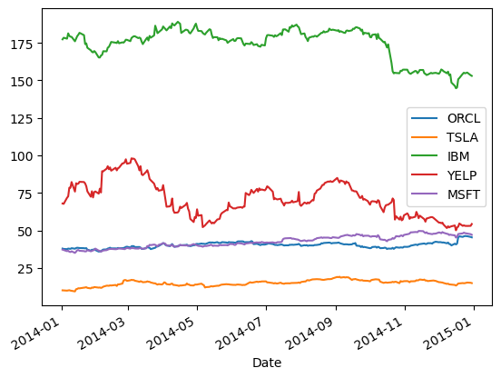
Comparing multiple stocks#

As a last task, we will use the experience we obtained so far – and learn some new things – in order to compare the performance of different stocks we obtained from Yahoo finance.

stocks = ['ORCL', 'TSLA', 'IBM','YELP', 'MSFT']
stock_df = pd.DataFrame()
for s in stocks:
    stock_df[s] = pd.DataFrame(yf.download(s,start='2014-01-01',end='2014-12-31', progress = False))['Close']
stock_df.head()

	ORCL	TSLA	IBM	YELP	MSFT
Date
2014-01-02	37.840000	10.006667	177.370941	67.919998	37.160000
2014-01-03	37.619999	9.970667	178.432129	67.660004	36.910000
2014-01-06	37.470001	9.800000	177.820267	71.720001	36.130001
2014-01-07	37.849998	9.957333	181.367111	72.660004	36.410000
2014-01-08	37.720001	10.085333	179.703629	78.419998	35.759998

stock_df.plot();

_images/e154867c67ed856817eeeb050d89f4802c945d6616086508d87a708110a0d91a.png

Next, we will calculate returns over a period of length \(T,\) defined as:

\[ r(t) = \frac{f(t)-f(t-T)}{f(t)} \]

The returns can be computed with a simple DataFrame method pct_change(). Note that for the first \(T\) timesteps, this value is not defined (of course):

rets = stock_df.pct_change(30)
rets.iloc[25:35]

	ORCL	TSLA	IBM	YELP	MSFT
Date
2014-02-07	NaN	NaN	NaN	NaN	NaN
2014-02-10	NaN	NaN	NaN	NaN	NaN
2014-02-11	NaN	NaN	NaN	NaN	NaN
2014-02-12	NaN	NaN	NaN	NaN	NaN
2014-02-13	NaN	NaN	NaN	NaN	NaN
2014-02-14	0.003700	0.320653	-0.009918	0.321849	0.012379
2014-02-18	0.009304	0.361995	-0.018485	0.355897	0.013817
2014-02-19	0.010675	0.317279	-0.016398	0.254880	0.038195
2014-02-20	0.011096	0.405798	-0.028728	0.257501	0.036803
2014-02-21	0.010074	0.385510	-0.027558	0.170875	0.062081

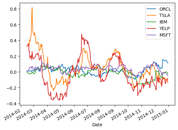
Now we’ll plot the timeseries of the returns of the different stocks.

Notice that the NaN values are gracefully dropped by the plotting function.

rets.plot();

_images/6b36dd35f5f7f66a5d8600ae1f0c0732df24177581c8be3516a20ffa5fc1023e.png

plt.scatter(rets.TSLA, rets.YELP)
plt.xlabel('TESLA 30-day returns')
plt.ylabel('YELP 30-day returns');

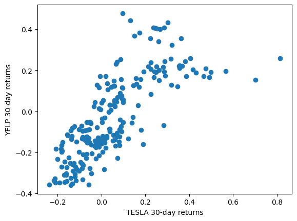
_images/27f083d0adb013b42c2f5197155dca5ea7765b67653522383d9743e81d592f21.png

There appears to be some (fairly strong) correlation between the movement of TSLA and YELP stocks. Let’s measure this.

The correlation coefficient between variables \(X\) and \(Y\) is defined as follows:

\[ \text{Corr}(X,Y) = \frac{E\left[(X-\mu_X)(Y-\mu_Y)\right]}{\sigma_X\sigma_Y} \]

Pandas provides a dataframe method to compute the correlation coefficient of all pairs of columns: corr().

rets.corr()

	ORCL	TSLA	IBM	YELP	MSFT
ORCL	1.000000	0.007218	0.026666	-0.083688	0.131830
TSLA	0.007218	1.000000	0.196371	0.769623	0.411348
IBM	0.026666	0.196371	1.000000	0.104705	0.343697
YELP	-0.083688	0.769623	0.104705	1.000000	0.264703
MSFT	0.131830	0.411348	0.343697	0.264703	1.000000

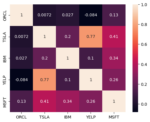
It takes a bit of time to examine that table and draw conclusions.

To speed that process up it helps to visualize the table.

We will learn more about visualization later, but for now this is a simple example.

sns.heatmap(rets.corr(), annot=True);

_images/734b13b0c632caf6c81005ca5a91be433ce0a00e15f423b6e9a88aa801680e94.png

Finally, it is important to know that the plotting performed by Pandas is just a layer on top of matplotlib (i.e., the plt package).

So Panda’s plots can (and often should) be replaced or improved by using additional functions from matplotlib.

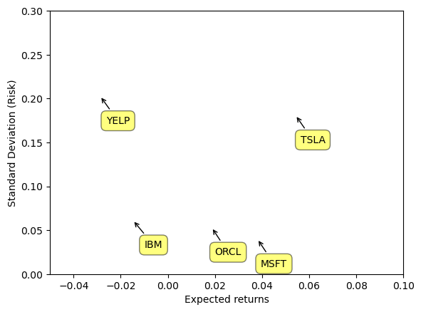
For example, suppose we want to know both the returns as well as the standard deviation of the returns of a stock (i.e., its risk).

Here is visualization of the result of such an analysis, and we construct the plot using only functions from matplotlib.

# plt.scatter(rets.mean(), rets.std());
plt.xlabel('Expected returns')
plt.ylabel('Standard Deviation (Risk)')
plt.xlim([-.05,.1])
plt.ylim([0,.3])
for label, x, y in zip(rets.columns, rets.mean(), rets.std()):
    plt.annotate(
        label, 
        xy = (x, y), xytext = (30, -30),
        textcoords = 'offset points', ha = 'right', va = 'bottom',
        bbox = dict(boxstyle = 'round,pad=0.5', fc = 'yellow', alpha = 0.5),
        arrowprops = dict(arrowstyle = '->', connectionstyle = 'arc3,rad=0'))

_images/26d1bc3889f0ace9b14130be6d894b78f098f2229bac7c0be9ab5fa7a29919af.png

To understand what these functions are doing, (especially the annotate function), you will need to consult the online documentation for matplotlib. Just use Google to find it.