Show code cell source
import numpy as np
import scipy as sp
import matplotlib.pyplot as plt
import pandas as pd
import sklearn.datasets as sk_data
from sklearn.cluster import KMeans

#import matplotlib as mpl
import seaborn as sns
%matplotlib inline
Hierarchical Clustering#
Today we will look at a fairly different approach to clustering.
So far, we have been thinking of clustering as finding a partition of our dataset.
That is, a set of nonoverlapping clusters, in which each data item is in one cluster.
However, in many cases, the notion of a strict partition is not as useful.
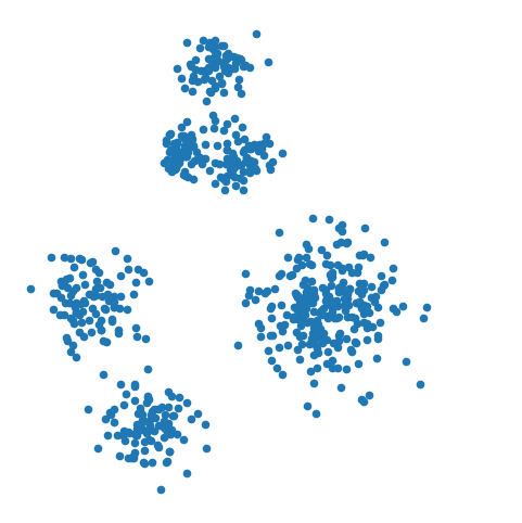
How Many Clusters?#
How many clusters would you say there are here?
Show code cell source
X_rand, y_rand = sk_data.make_blobs(n_samples=[100, 100, 250, 70, 75, 80], centers = [[1, 2], [1.5, 1], [3, 2], [1.75, 3.25], [2, 4], [2.25, 3.25]], n_features = 2,
                          center_box = (-10.0, 10.0), cluster_std = [.2, .2, .3, .1, .15, .15], random_state = 0)
df_rand = pd.DataFrame(np.column_stack([X_rand[:, 0], X_rand[:, 1], y_rand]), columns = ['X', 'Y', 'label'])
df_rand = df_rand.astype({'label': 'int'})
df_rand['label2'] = [{0: 0, 1: 1, 2: 2, 3: 3, 4: 3, 5: 3}[x] for x in df_rand['label']]
df_rand['label3'] = [{0: 0, 1: 0, 2: 1, 3: 2, 4: 2, 5: 2}[x] for x in df_rand['label']]
# kmeans = KMeans(init = 'k-means++', n_clusters = 3, n_init = 100)
# df_rand['label'] = kmeans.fit_predict(df_rand[['X', 'Y']])
Show code cell source
df_rand.plot('X', 'Y', kind = 'scatter', colormap='viridis',
                   colorbar = False, figsize = (6, 6))
plt.axis('square')
plt.axis('off');
/Users/crovella/miniconda3/lib/python3.9/site-packages/pandas/plotting/_matplotlib/core.py:1259: UserWarning: No data for colormapping provided via 'c'. Parameters 'cmap' will be ignored
  scatter = ax.scatter(
Three clusters?
Show code cell source
df_rand.plot('X', 'Y', kind = 'scatter', c = 'label3', colormap='viridis',
                   colorbar = False, figsize = (6, 6))
plt.axis('square')
plt.axis('off');
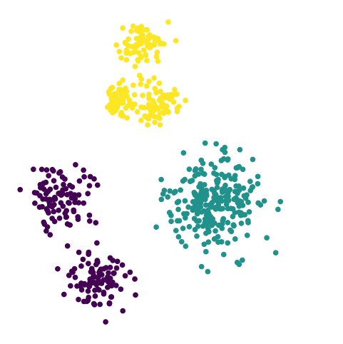
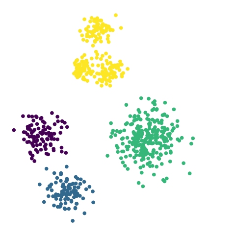
Four clusters?
Show code cell source
df_rand.plot('X', 'Y', kind = 'scatter', c = 'label2', colormap='viridis',
                   colorbar = False, figsize = (6, 6))
plt.axis('square')
plt.axis('off');
Six clusters?
Show code cell source
df_rand.plot('X', 'Y', kind = 'scatter', c = 'label', colormap='viridis',
                   colorbar = False, figsize = (6, 6))
plt.axis('square')
plt.axis('off');
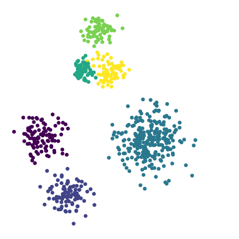
This dataset shows clustering on multiple scales.
To fully capture the structure in this dataset, two things are needed:
Capturing the differing clusters depending on the scale
Capturing the containment relations – which clusters lie within other clusters
These observations motivate the notion of hierarchical clustering.
In hierarchical clustering, we move away from the partition notion of \(k\)-means,
and instead capture a more complex arrangement that includes containment of one cluster within another.
Hierarchical Clustering#
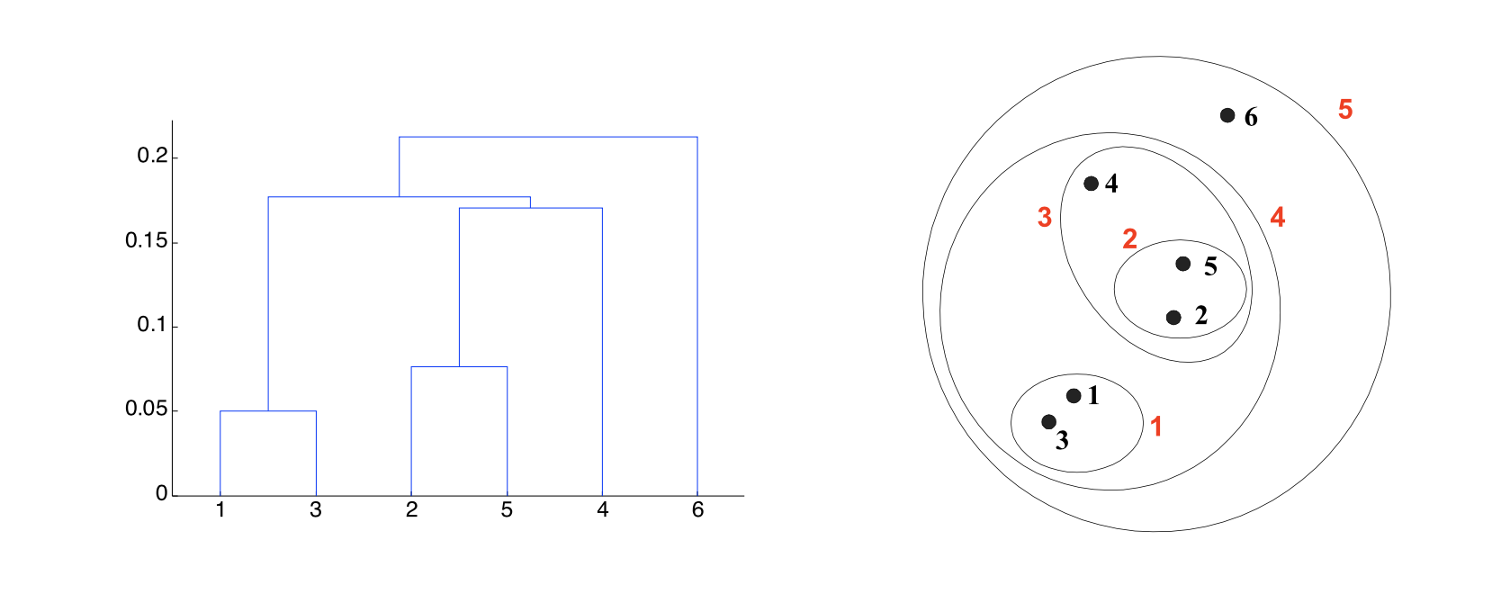
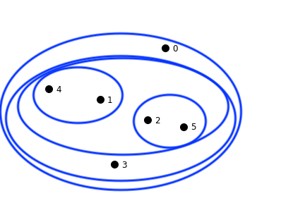
A hierarchical clustering produces a set of nested clusters organized into a tree.
A hierarchical clustering is visualized using a dendrogram
A tree-like diagram that records the containment relations among clusters.
Strengths of Hierarchical Clustering#
Hierarchical clustering has a number of advantages:
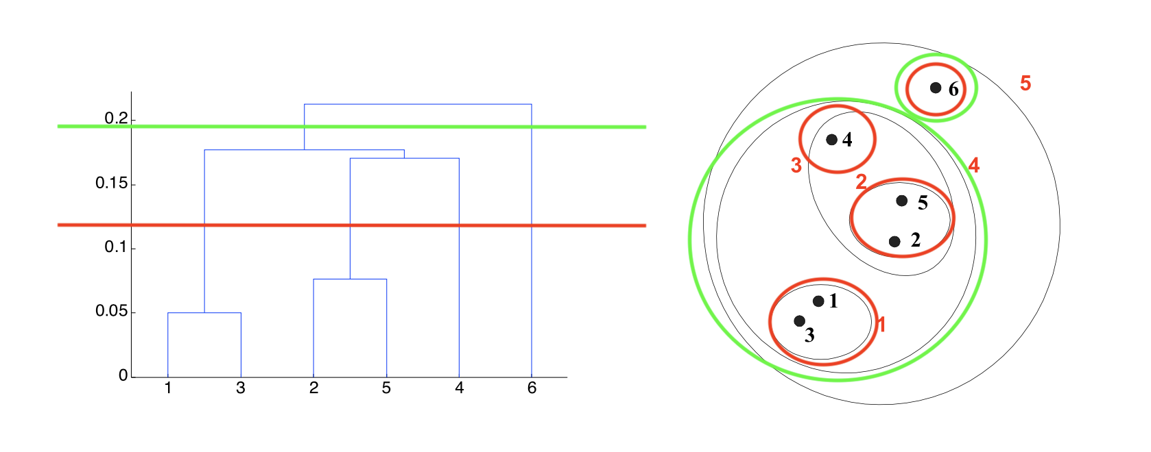
First, a hierarchical clustering encodes many different clusterings. That is, it does not itself decide on the correct number of clusters.
A clustering is obtained by “cutting” the dendrogram at some level.
This means that you can make this crucial decision yourself, by inspecting the dendrogram.
Put another way, you can obtain any desired number of clusters.
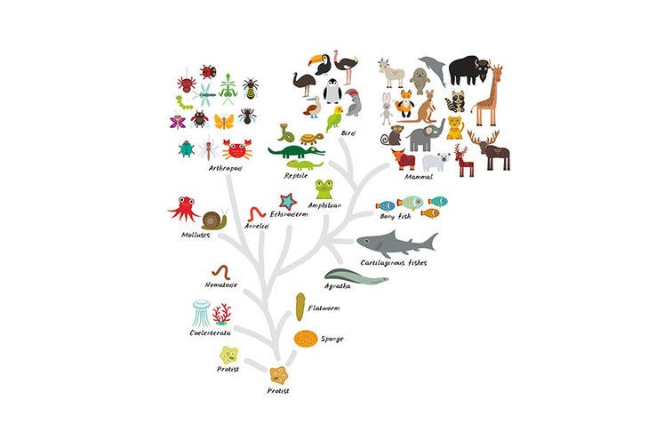
The second advantage is that the dendrogram may itself correspond to a meaningful structure, for example, a taxonomy.
The third advantage is that many hierarchical clustering methods can be performed using either similarity (proximity) or dissimilarity (distance) metrics.
This can be very helpful!
(Note that techniques like \(k\)-means cannot be used with unmodified similarity metrics.)
Compared to \(k\)-means#
Another aspect of hierachical clustering is that it can handle certain cases better than \(k\)-means.
Because of the nature of the \(k\)-means algorithm, \(k\)-means tends to produce:
Roughly spherical clusters
Clusters of approximately equal size
Non-overlapping clusters
In many real-world situations, clusters may not be round, they may be of unequal size, and they may overlap.
Hence we would like clustering algorithms that can work in those cases also.
Hierarchical Clustering Algorithms#
There are two main approaches to hierarchical clustering: “bottom-up” and “top-down.”
Agglomerative Clustering (“bottom-up”):
Start by defining each point as its own cluster
At each successive step, merge the two clusters that are closest to each other
Repeat until only one cluster is left.
Divisive Clustering (“top-down”):
Start with one, all-inclusive cluster
At each step, find the cluster split that creates the largest distance between resulting clusters
Repeat until each point is in its own cluster.
Agglomerative techniques are by far the more common.
The key to both of these methods is defining the distance between two clusters.
Different definitions for the inter-cluster distance yield different clusterings.
To illustrate the impact of the choice of cluster distances, we’ll focus on agglomerative clustering.
Defining Cluster Proximity#
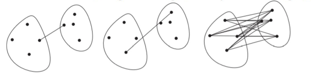
Given two clusters, how do we define the distance between them?
Here are three natural ways to do it:
Single-Linkage: the distance between two clusters is the distance between the closest two points that are in different clusters.
Complete-Linkage: the distance between two clusters is the distance between the farthest two points that are in different clusters.
Average-Linkage: the distance between two clusters is the average distance between all pairs of points from different clusters.
Notice that it is easy to express the definitions above in terms of similarity instead of distance.
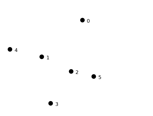
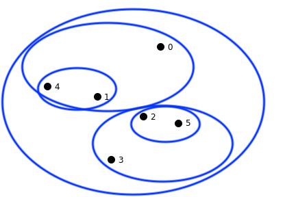
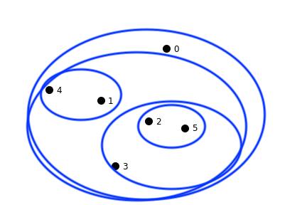
Here is a set of 6 points that we will cluster to show differences between distance metrics.
Show code cell source
pt_x = [0.4, 0.22, 0.35, 0.26, 0.08, 0.45]
pt_y = [0.53, 0.38, 0.32, 0.19, 0.41, 0.30]
plt.plot(pt_x, pt_y, 'o', markersize = 10, color = 'k')
plt.ylim([.15, .60])
plt.xlim([0.05, 0.70])
for i in range(6):
    plt.annotate(f'{i}', (pt_x[i]+0.02, pt_y[i]-0.01), fontsize = 12)
plt.axis('off')
plt.savefig('figs/L08-basic-pointset.png');
Show code cell source
X = np.array([pt_x, pt_y]).T
from scipy.spatial import distance_matrix
labels = ['p0', 'p1', 'p2', 'p3', 'p4', 'p5']
D = pd.DataFrame(distance_matrix(X, X), index = labels, columns = labels)
D.style.format('{:.2f}')
| p0 | p1 | p2 | p3 | p4 | p5 | |
|---|---|---|---|---|---|---|
| p0 | 0.00 | 0.23 | 0.22 | 0.37 | 0.34 | 0.24 |
| p1 | 0.23 | 0.00 | 0.14 | 0.19 | 0.14 | 0.24 |
| p2 | 0.22 | 0.14 | 0.00 | 0.16 | 0.28 | 0.10 |
| p3 | 0.37 | 0.19 | 0.16 | 0.00 | 0.28 | 0.22 |
| p4 | 0.34 | 0.14 | 0.28 | 0.28 | 0.00 | 0.39 |
| p5 | 0.24 | 0.24 | 0.10 | 0.22 | 0.39 | 0.00 |
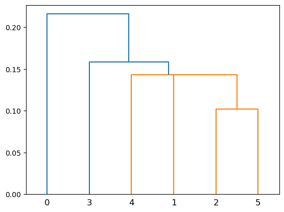
Single-Linkage Clustering#
Show code cell source
import scipy.cluster
import scipy.cluster.hierarchy as hierarchy
Z = hierarchy.linkage(X, method='single')
hierarchy.dendrogram(Z);
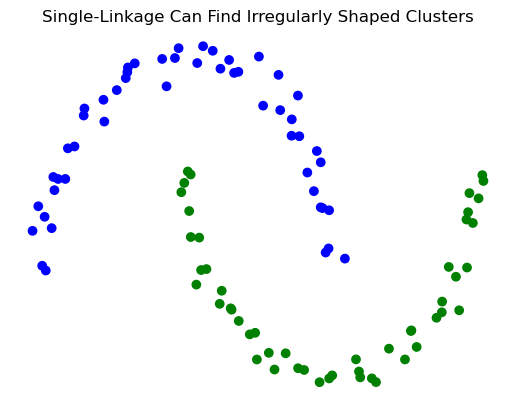
Advantages:
Single-linkage clustering can handle non-elliptical shapes.
In fact it can produce long, elongated clusters:
Show code cell source
X_moon_05, y_moon_05 = sk_data.make_moons(random_state = 0, noise = 0.05)
Z = hierarchy.linkage(X_moon_05, method='single')
labels = hierarchy.fcluster(Z, 2, criterion = 'maxclust')
plt.scatter(X_moon_05[:,0], X_moon_05[:,1], c = [['b','g'][i-1] for i in labels])
plt.title('Single-Linkage Can Find Irregularly Shaped Clusters')
plt.axis('off');
Show code cell source
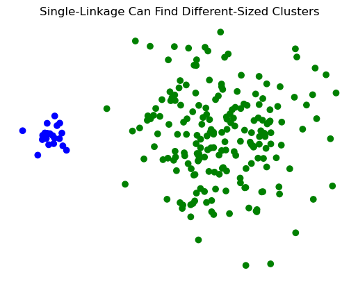
X_rand_lo, y_rand_lo = sk_data.make_blobs(n_samples=[20, 200], centers = [[1, 1], [3, 1]], n_features = 2,
                          center_box = (-10.0, 10.0), cluster_std = [.1, .5], random_state = 0)
Z = hierarchy.linkage(X_rand_lo, method='single')
labels = hierarchy.fcluster(Z, 2, criterion = 'maxclust')
plt.scatter(X_rand_lo[:,0], X_rand_lo[:,1], c = [['b','g'][i-1] for i in labels])
plt.title('Single-Linkage Can Find Different-Sized Clusters')
plt.axis('off');
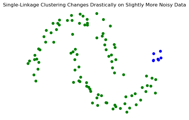
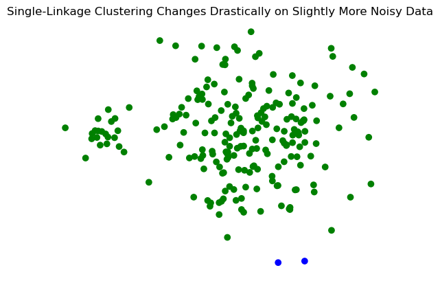
Disadvantages:
Single-linkage clustering can be sensitive to noise and outliers.
Show code cell source
X_moon_10, y_moon_10 = sk_data.make_moons(random_state = 0, noise = 0.1)
Z = hierarchy.linkage(X_moon_10, method='single')
labels = hierarchy.fcluster(Z, 2, criterion = 'maxclust')
plt.scatter(X_moon_10[:,0], X_moon_10[:,1], c = [['b','g'][i-1] for i in labels])
plt.title('Single-Linkage Clustering Changes Drastically on Slightly More Noisy Data')
plt.axis('off');
Show code cell source
X_rand_hi, y_rand_hi = sk_data.make_blobs(n_samples=[20, 200], centers = [[1, 1], [3, 1]], n_features = 2,
                          center_box = (-10.0, 10.0), cluster_std = [.15, .6], random_state = 0)
Z = hierarchy.linkage(X_rand_hi, method='single')
labels = hierarchy.fcluster(Z, 2, criterion = 'maxclust')
plt.title('Single-Linkage Clustering Changes Drastically on Slightly More Noisy Data')
plt.scatter(X_rand_hi[:,0], X_rand_hi[:,1], c = [['b','g'][i-1] for i in labels])
plt.axis('off');
Complete-Linkage Clustering#
Show code cell source
Z = hierarchy.linkage(X, method='complete')
hierarchy.dendrogram(Z);
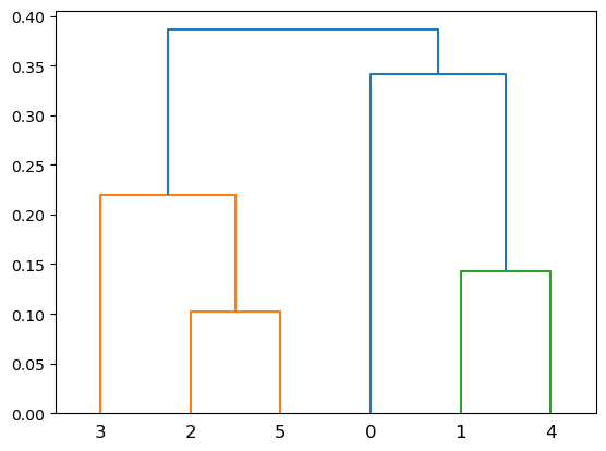
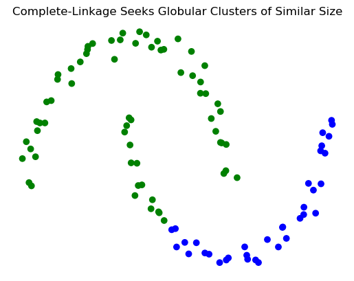
Advantages:
Produces more-balanced clusters – more-equal diameters
Show code cell source
X_moon_05, y_moon_05 = sk_data.make_moons(random_state = 0, noise = 0.05)
Z = hierarchy.linkage(X_moon_05, method='complete')
labels = hierarchy.fcluster(Z, 2, criterion = 'maxclust')
plt.scatter(X_moon_05[:,0], X_moon_05[:,1], c = [['b','g'][i-1] for i in labels])
plt.title('Complete-Linkage Seeks Globular Clusters of Similar Size')
plt.axis('off');
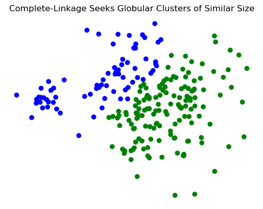
Show code cell source
Z = hierarchy.linkage(X_rand_hi, method='complete')
labels = hierarchy.fcluster(Z, 2, criterion = 'maxclust')
plt.scatter(X_rand_hi[:,0], X_rand_hi[:,1], c = [['b','g'][i-1] for i in labels])
plt.title('Complete-Linkage Seeks Globular Clusters of Similar Size')
plt.axis('off');
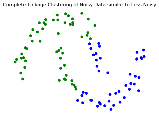
Less susceptible to noise:
Show code cell source
Z = hierarchy.linkage(X_moon_10, method='complete')
labels = hierarchy.fcluster(Z, 2, criterion = 'maxclust')
plt.scatter(X_moon_10[:,0], X_moon_10[:,1], c = [['b','g'][i-1] for i in labels])
plt.title('Complete-Linkage Clustering of Noisy Data similar to Less Noisy')
plt.axis('off');
Average-Linkage Clustering#
Show code cell source
Z = hierarchy.linkage(X, method='average')
hierarchy.dendrogram(Z);
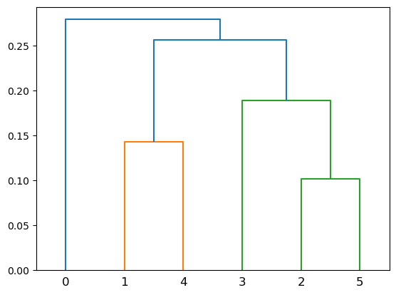
Average-Linkage clustering is in some sense a compromise between Single-linkage and Complete-linkage clustering.
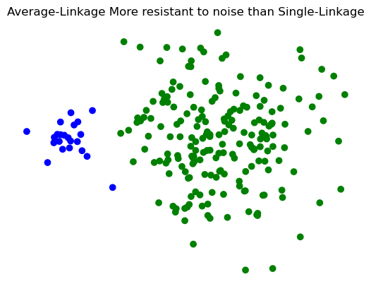
Strengths:
Less susceptible to noise and outliers
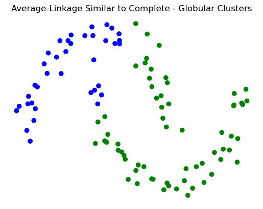
Limitations:
Biased toward elliptical clusters
Show code cell source
Z = hierarchy.linkage(X_moon_10, method='average')
labels = hierarchy.fcluster(Z, 2, criterion = 'maxclust')
plt.scatter(X_moon_10[:,0], X_moon_10[:,1], c = [['b','g'][i-1] for i in labels])
plt.title('Average-Linkage Similar to Complete - Globular Clusters')
plt.axis('off');
Show code cell source
Z = hierarchy.linkage(X_rand_hi, method='average')
labels = hierarchy.fcluster(Z, 2, criterion = 'maxclust')
plt.scatter(X_rand_hi[:,0], X_rand_hi[:,1], c = [['b','g'][i-1] for i in labels])
plt.title('Average-Linkage More resistant to noise than Single-Linkage')
plt.axis('off');
All Three Compared#
 Single-Linkage
 Complete-Linkage
 Average-Linkage
Ward’s Distance#
Finally, we consider one more cluster distance.
Ward’s distance asks “what if”.
That is, “What if we combined these two clusters – how would clustering improve?”
To define “how would clustering improve?” we appeal to the \(k\)-means criterion.
So:
Ward’s Distance between clusters \(C_i\) and \(C_j\) is the difference between the total within cluster sum of squares for the two clusters separately, compared to the within cluster sum of squares resulting from merging the two clusters into a new cluster \(C_{i+j}\):
where \(r_i, r_j, r_{i+j}\) are the corresponding cluster centroids.
In a sense, this cluster distance results in a hierarchical analog of \(k\)-means.
As a result, it has properties similar to \(k\)-means:
Less susceptible to noise and outliers
Biased toward elliptical clusters
Hence it tends to behave more like group-average hierarchical clustering.
Hierarchical Clustering In Practice#
Now we’ll look at doing hierarchical clustering in practice, using python.
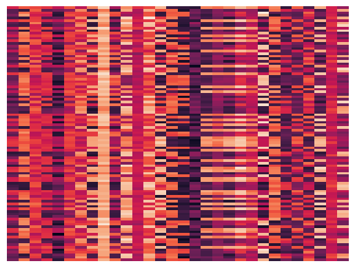
We’ll use the same synthetic data as we did in the k-means case – ie., three “blobs” living in 30 dimensions.
X, y = sk_data.make_blobs(n_samples=100, centers=3, n_features=30,
                          center_box=(-10.0, 10.0),random_state=0)
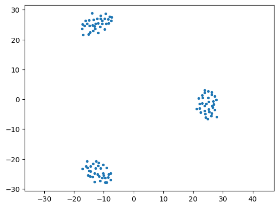
As a reminder of the raw data here is the visualization: first the raw data, then an embedding into 2-D (using MDS).
sns.heatmap(X, xticklabels=False, yticklabels=False, linewidths=0,cbar=False);
import sklearn.manifold
import sklearn.metrics as metrics
euclidean_dists = metrics.euclidean_distances(X)
mds = sklearn.manifold.MDS(n_components = 2, max_iter = 3000, eps = 1e-9, random_state = 0,
                   dissimilarity = "precomputed", n_jobs = 1)
fit = mds.fit(euclidean_dists)
pos = fit.embedding_
plt.axis('equal')
plt.scatter(pos[:, 0], pos[:, 1], s = 8);
/Users/crovella/miniconda3/lib/python3.9/site-packages/sklearn/manifold/_mds.py:299: FutureWarning: The default value of `normalized_stress` will change to `'auto'` in version 1.4. To suppress this warning, manually set the value of `normalized_stress`.
  warnings.warn(
Hierarchical clustering is available in sklearn, but there is a much more fully developed set of tools in the scipy package and that is the one to use.
import scipy.cluster
import scipy.cluster.hierarchy as hierarchy
import scipy.spatial.distance
# linkages = ['single','complete','average','weighted','ward']
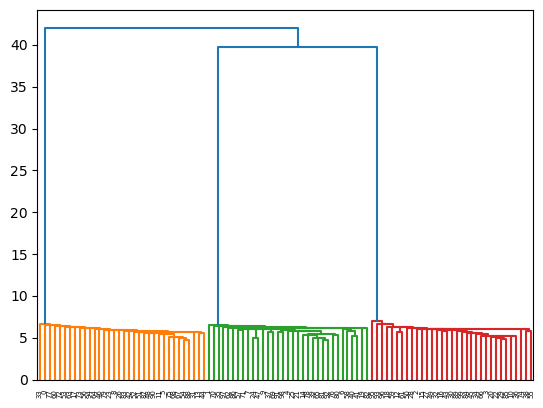
Z = hierarchy.linkage(X, method = 'single')
R = hierarchy.dendrogram(Z)
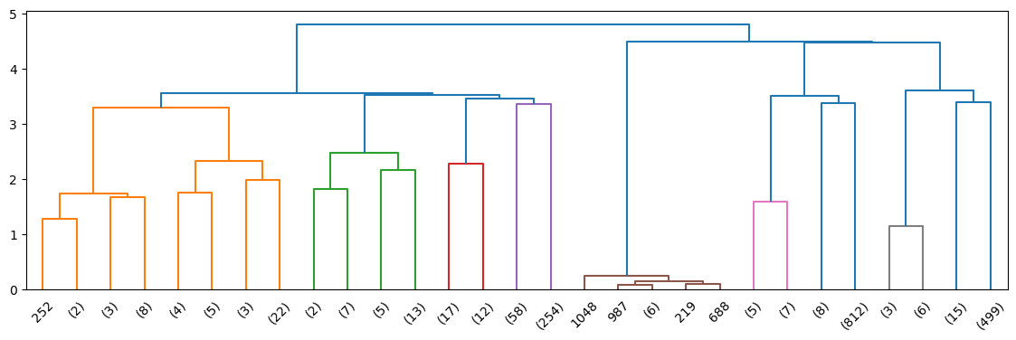
Hierarchical Clustering Real Data#
Once again we’ll use the “20 Newsgroup” data provided as example data in sklearn.
(http://scikit-learn.org/stable/datasets/twenty_newsgroups.html).
from sklearn.datasets import fetch_20newsgroups
categories = ['comp.os.ms-windows.misc', 'sci.space','rec.sport.baseball']
news_data = fetch_20newsgroups(subset = 'train', categories = categories)
from sklearn.feature_extraction.text import TfidfVectorizer
vectorizer = TfidfVectorizer(stop_words='english', min_df = 4, max_df = 0.8)
data = vectorizer.fit_transform(news_data.data).todense()
data.shape
(1781, 9409)
# metrics can be ‘braycurtis’, ‘canberra’, ‘chebyshev’, ‘cityblock’, ‘correlation’, ‘cosine’,
# ‘dice’, ‘euclidean’, ‘hamming’, ‘jaccard’, ‘kulsinski’, ‘mahalanobis’, ‘matching’,
# ‘minkowski’, ‘rogerstanimoto’, ‘russellrao’, ‘seuclidean’, ‘sokalmichener’, ‘sokalsneath’,
# ‘sqeuclidean’, ‘yule’.
Z_20ng = hierarchy.linkage(data, method = 'ward', metric = 'euclidean')
plt.figure(figsize=(14,4))
R_20ng = hierarchy.dendrogram(Z_20ng, p=4, truncate_mode = 'level', show_leaf_counts=True)
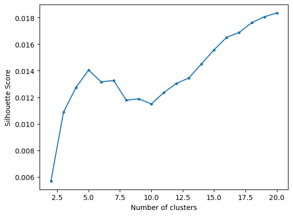
Selecting the Number of Clusters#
clusters = hierarchy.fcluster(Z_20ng, 3, criterion = 'maxclust')
print(clusters.shape)
clusters
(1781,)
array([3, 3, 3, ..., 1, 3, 1], dtype=int32)
max_clusters = 20
s = np.zeros(max_clusters+1)
for k in range(2, max_clusters+1):
    clusters = hierarchy.fcluster(Z_20ng, k, criterion = 'maxclust')
    s[k] = metrics.silhouette_score(np.asarray(data), clusters, metric = 'euclidean')
plt.plot(range(2, len(s)), s[2:], '.-')
plt.xlabel('Number of clusters')
plt.ylabel('Silhouette Score');
print('Top Terms Per Cluster:')
k = 5
clusters = hierarchy.fcluster(Z_20ng, k, criterion = 'maxclust')
for i in range(1,k+1):
    items = np.array([item for item,clust in zip(data, clusters) if clust == i])
    centroids = np.squeeze(items).mean(axis = 0)
    asc_order_centroids = centroids.argsort()#[:, ::-1]
    order_centroids = asc_order_centroids[::-1]
    terms = vectorizer.get_feature_names_out()
    print(f'Cluster {i}:')
    for ind in order_centroids[:10]:
        print(f' {terms[ind]}')
    print('')
Top Terms Per Cluster:
Cluster 1:
 space
 nasa
 edu
 henry
 gov
 alaska
 access
 com
 moon
 digex

Cluster 2:
 ax
 max
 b8f
 g9v
 a86
 145
 1d9
 pl
 2di
 0t

Cluster 3:
 edu
 com
 year
 baseball
 article
 writes
 cs
 team
 game
 university

Cluster 4:
 risc
 instruction
 ghhwang
 csie
 set
 nctu
 cisc
 tw
 reduced
 mq

Cluster 5:
 windows
 edu
 file
 dos
 com
 files
 card
 drivers
 driver
 use