Decision Trees#
Today we start our study of classification methods.
Recall that in a classification problem, we have data tuples \((\mathbf{x}, y)\) in which the \(\mathbf{x}\) are the features, and the \(y\) values are categorical data.
We typically call the \(y\) values “labels” or “classes.”
Some examples of classification tasks:
Predicting tumor cells as malignant or benign
Classifying credit card transactions as legitimate or fraudulent
Classifying secondary structures of a protein as alpha-helix, beta-sheet, or other
Categorizing news stories as finance, weather, entertainment, sports, etc
The first classification method we will consider is called the decision tree.
It is a very popular method, and has some nice properties as we will see.
Decision Trees in Action#
We will start by describing how a decision tree works.
We are assuming a decision tree has been built to solve the following classification problem:
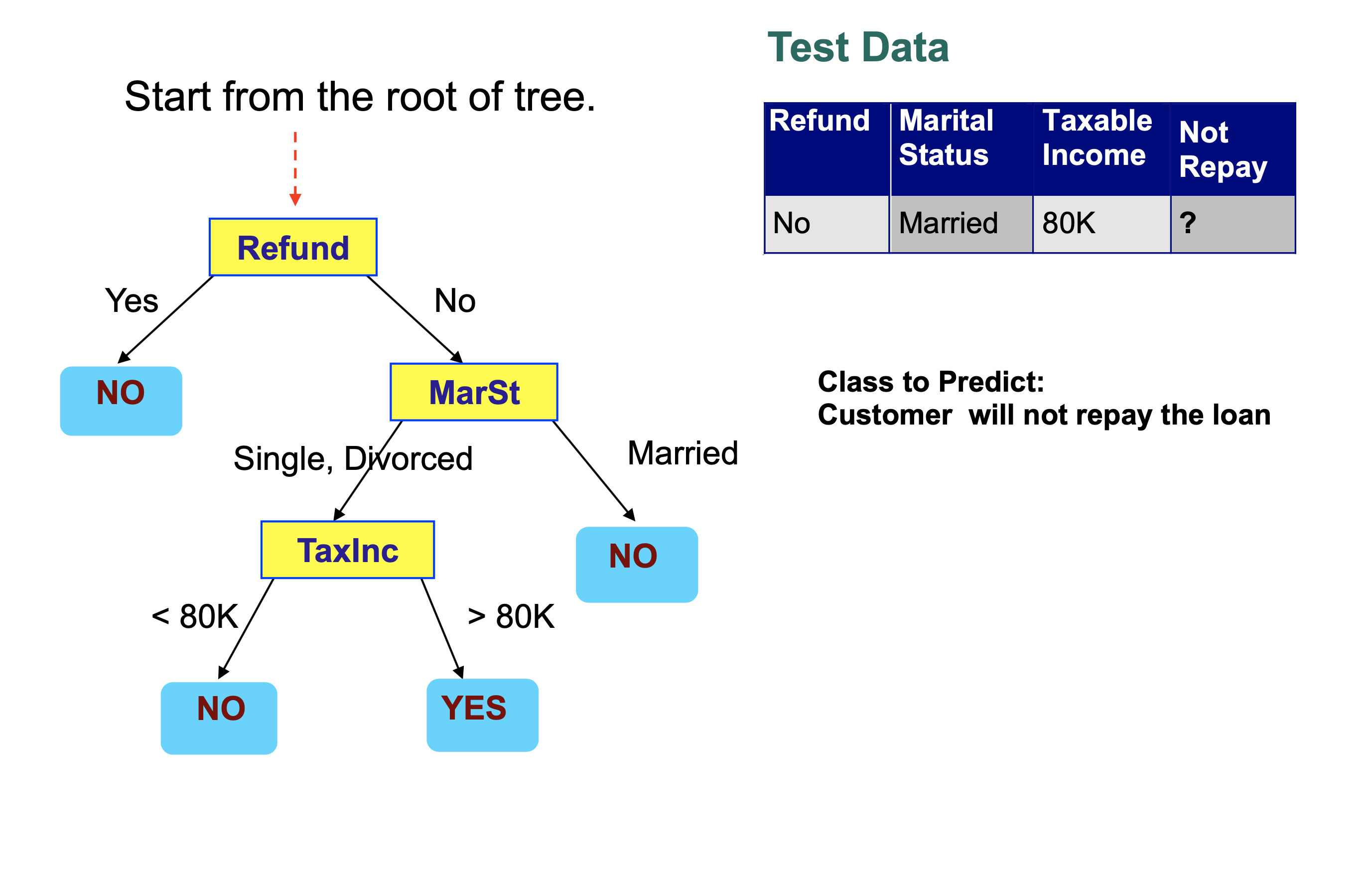
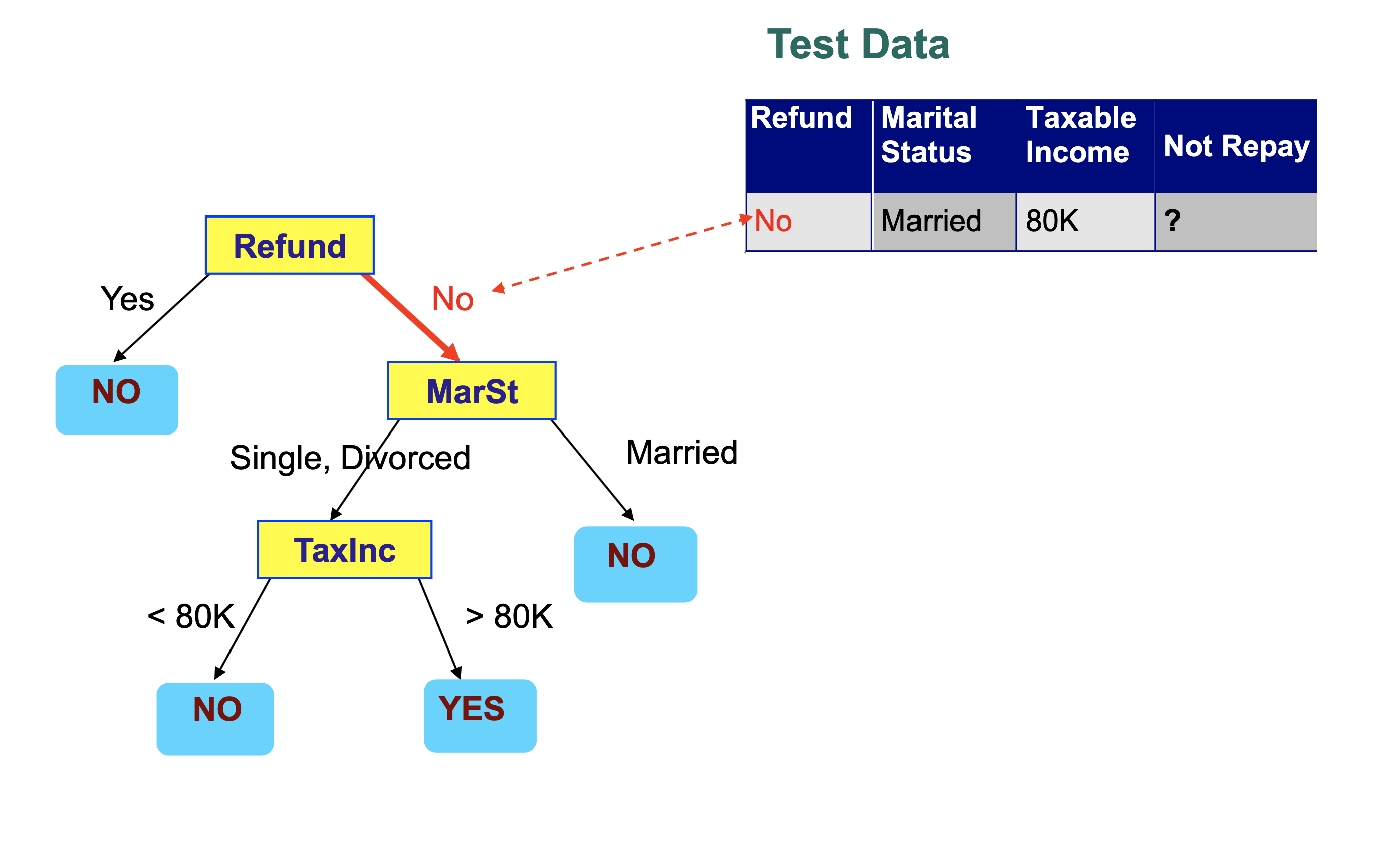
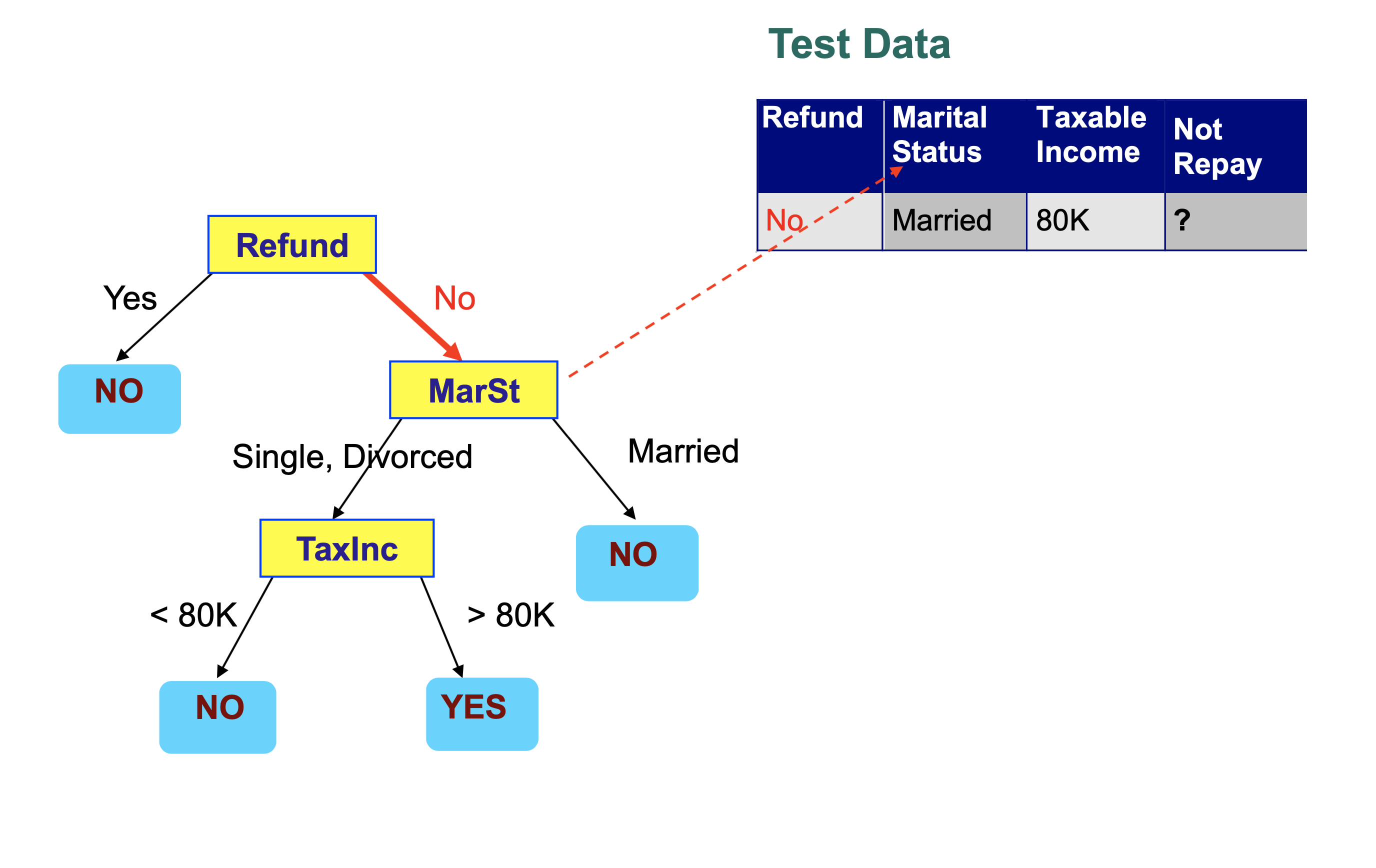
We then step through the tree, making a decision at each node that takes us to another node in the tree.
Each decision examines a single feature in the item being classified.

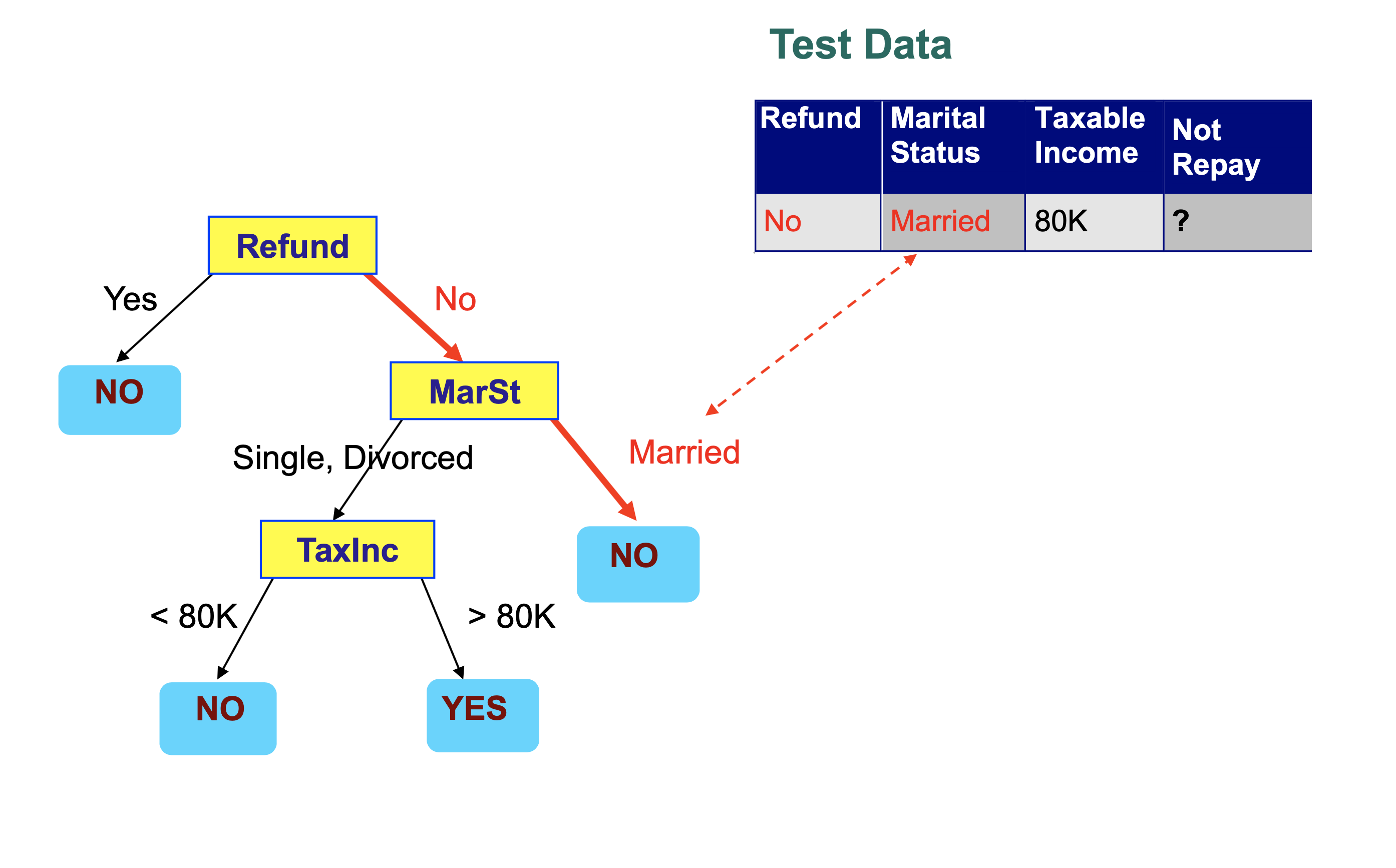
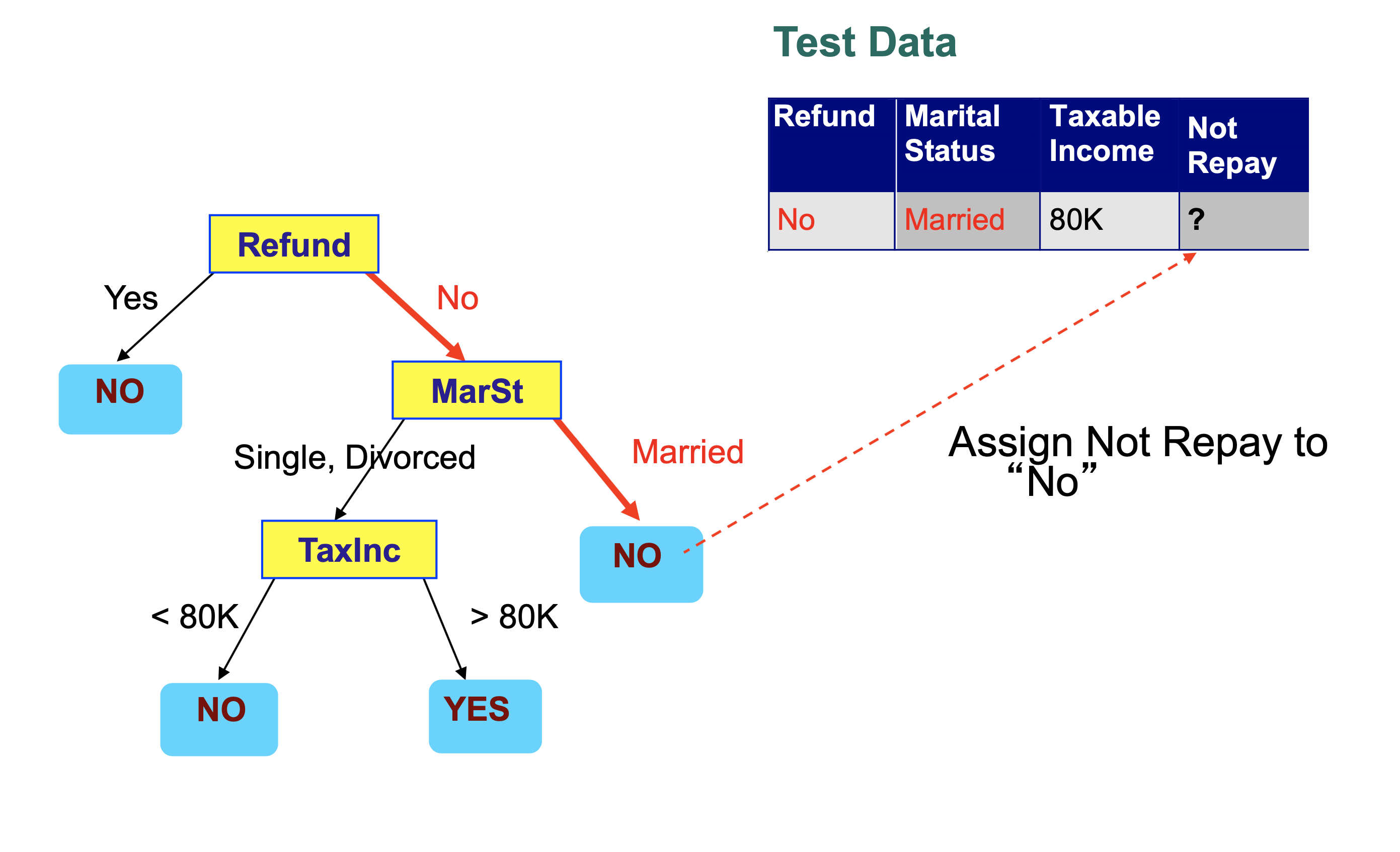
We conclude that this record is classified as “Not Repay” is “No”.
Note also that decision trees can be used to predict numeric values, so they are used for regression as well.
The general term “Classification and Regression Tree” (CART) is sometimes used – although this term also refers to a specific decision tree learning algorithm.
Learning a Decision Tree#
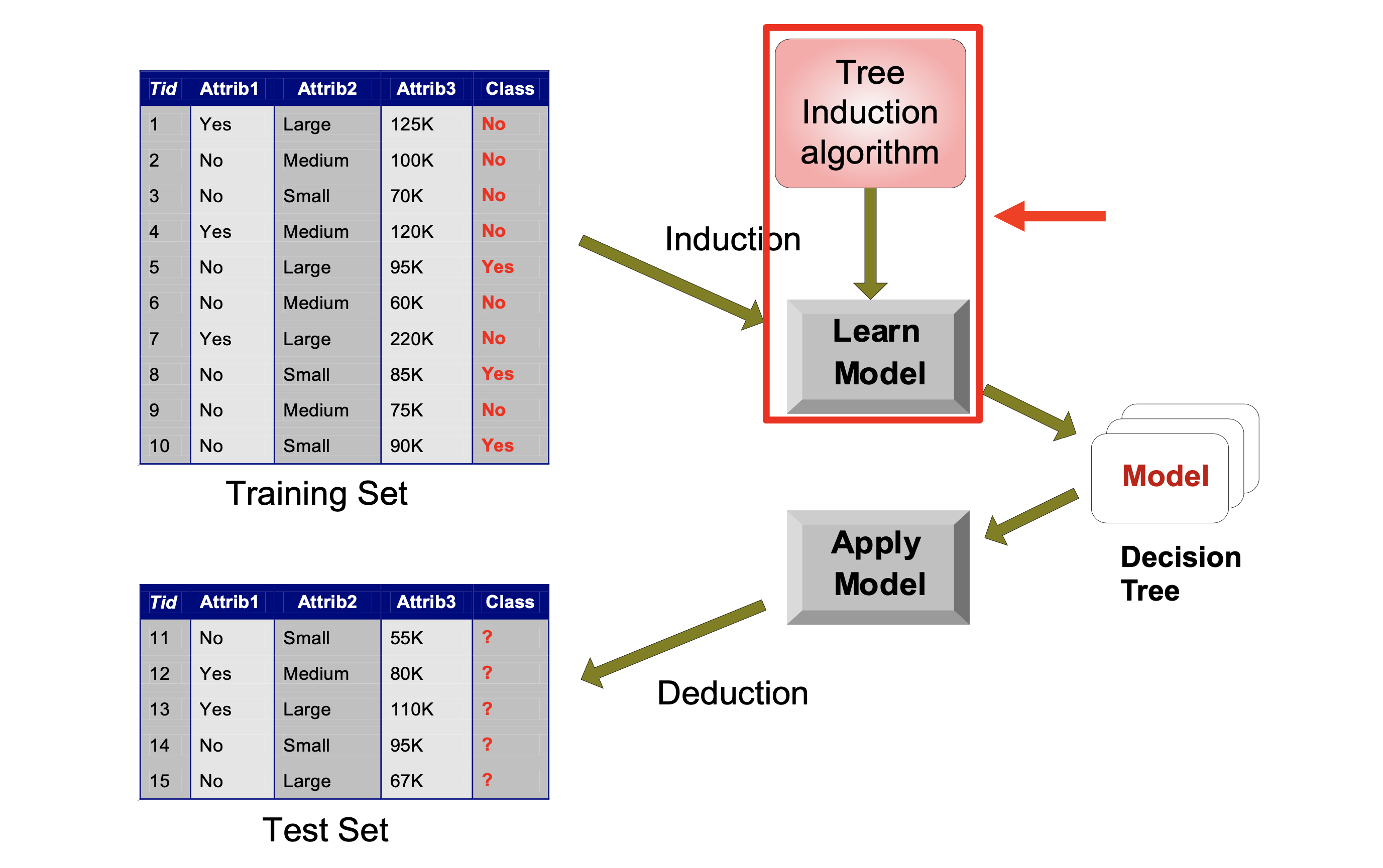
We’ve discussed how to apply a decision tree to data (lower portion of this figure).
But how does one train a decision tree? What algorithm can we use?
A number of algorithms have been proposed for building decision trees:
Hunt’s algorithm (one of the earliest)
CART
ID3, C4.5
SLIQ, SPRINT
etc
We will look at Hunt’s Algorithm as our example.
Hunt’s Algorithm#
Hunt’s Algorithm builds the tree node by node, starting from the root.
As we build the tree, we divide the training data up.
Let \(D_t\) be the set of training records that reach node \(t\).
If \(D_t\) contains records that all belong to a single class \(y_t\), then \(t\) is a leaf node labeled as \(y_t\).
If \(D_t\) is an empty set, then \(t\) is a leaf node labeled by the default class \(y_d\).
If \(D_t\) contains records that belong to more than one class, use an attribute to split \(D_t\) into smaller subsets, and assign that splitting-rule to node \(t\).
Recursively apply the above procedure until a stopping criterion is met.

So as Hunt’s algorithm progresses, records are divided up and assigned to leaf nodes. The most challenging step in Hunt’s algorithm is deciding which leaf node to split next, and how to specify the split.
In general, we use a greedy strategy. We will split a set of records based on an attribute test that optimizes some criterion.
We choose the set to split that provides the largest improvement in our criterion.
Once we have chosen the set to split, the remaining questions are:
Determining how to split the record set
How should we specify the attribute test condition?
How should we determine the best split for a set based on a given attribute?
Determining when to stop splitting.
Specifying the Test Condition#
How we specify a test condition depends on the attribute type:
Nominal (Categorical)
Ordinal (eg, Small, Medium, Large)
Continuous
And depends on the number of ways to split - multi-way or binary:
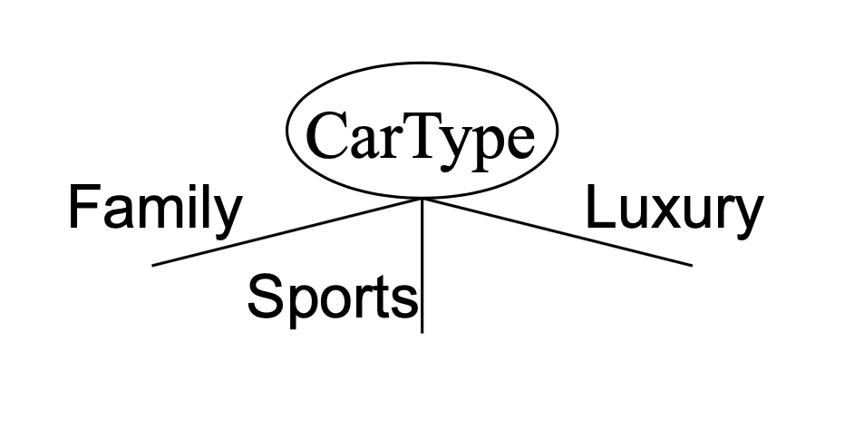
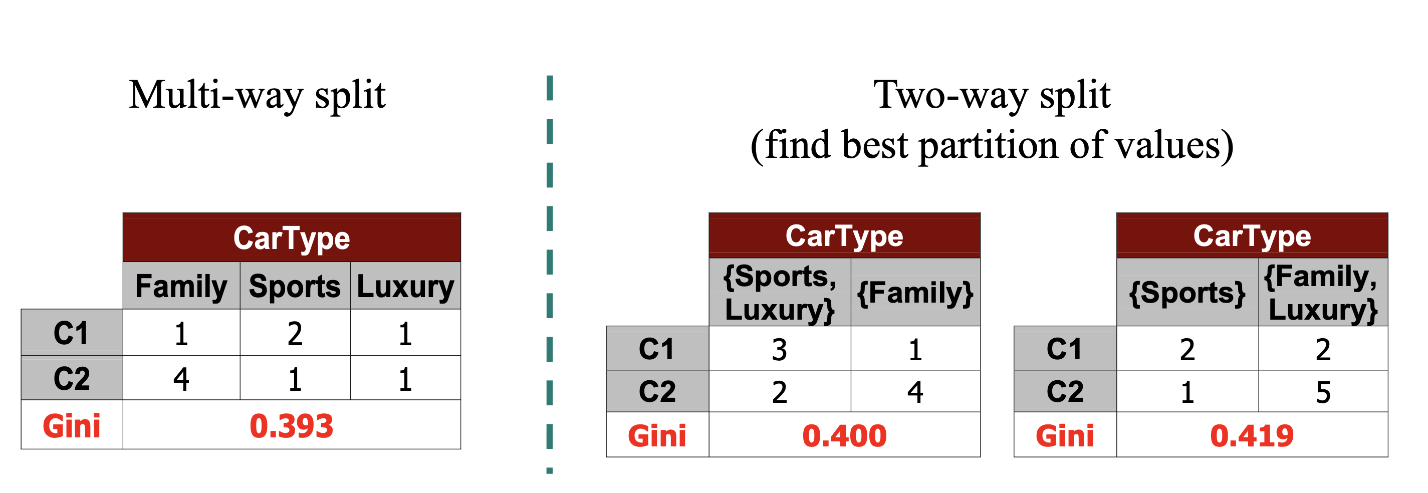
For a Nominal attribute:
In a Multi-way split we can use as many partitions as there are distinct values of the attribute:
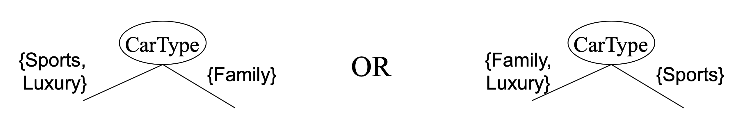
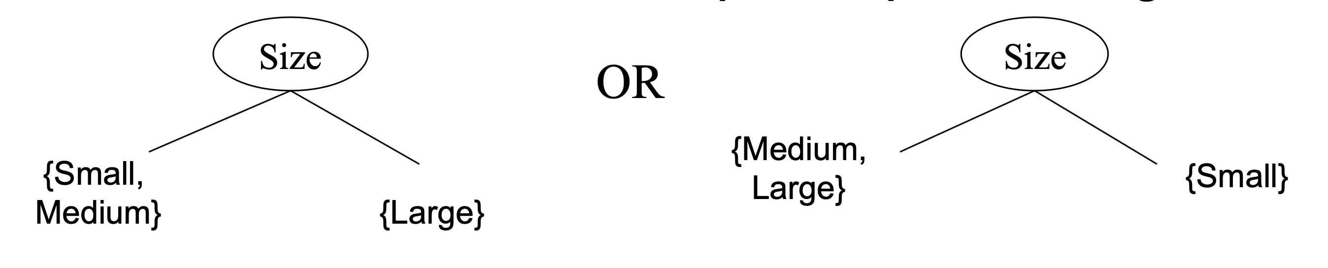
In a Binary split we divide the values into two groups. In this case, we need to find an optimal partitioning of values into groups.
An Ordinal attribute is similar to a Nominal attribute, except that since attributes have an ordering, we can specify the test in terms of a threshold. This simplifies the search for a good paritition.
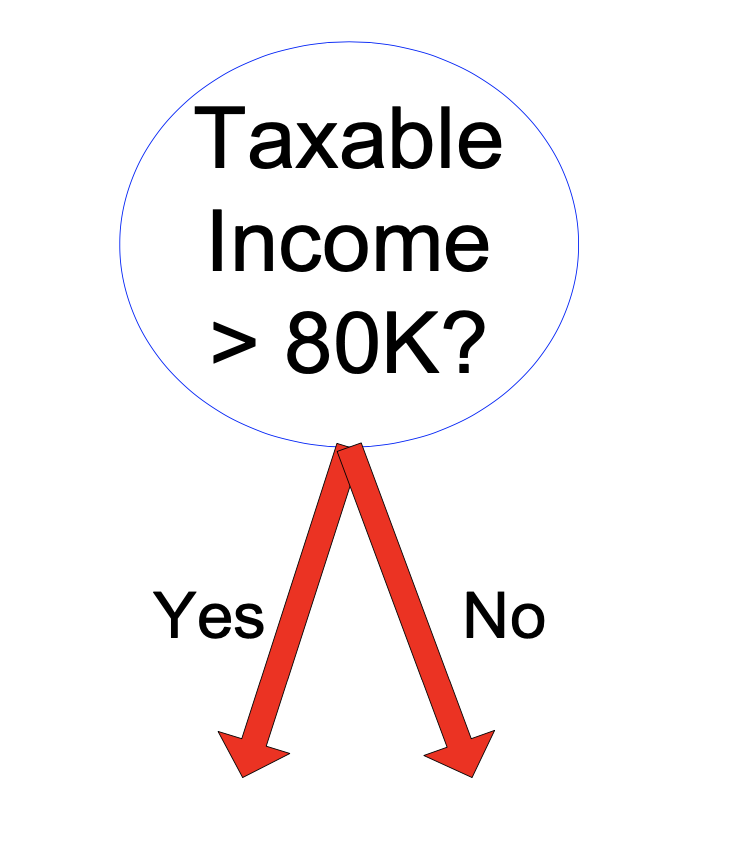
A Continuous attribute can be handled two ways:
It can be discretized to form an ordinal categorical attribute
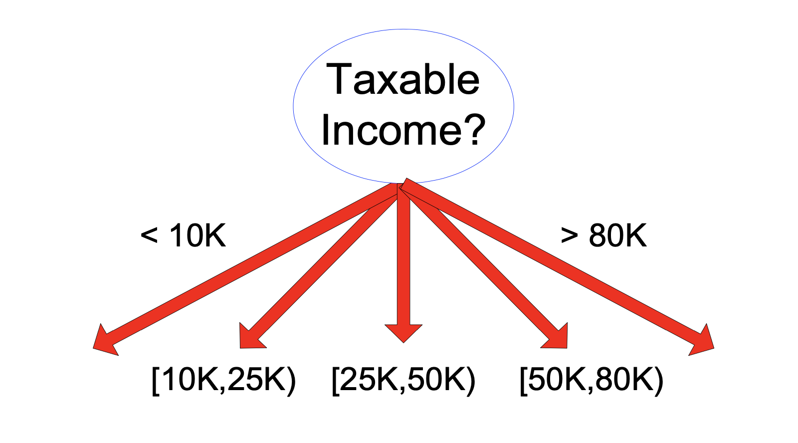
Or it can be partitioned via a threshold to form for a binary split.
Note that finding good partitions for nominal attributes can be expensive, possibly involving combinatorial searching of groupings.
However for ordinal or continuous attributes, sweeping through a range of threshold values can be more efficient.
Determining the Best Split#
Our algorithmic strategy is to split record sets so as to improve classification accuracy on the training data.
When is classification accuracy maximized?
When each leaf node contains records that all have the same label.
Consider this case:
At some node in the tree, before splitting that node’s records, we have
10 records from class 0, and
10 records from class 1
There are three attributes we can split on. Which split is best?
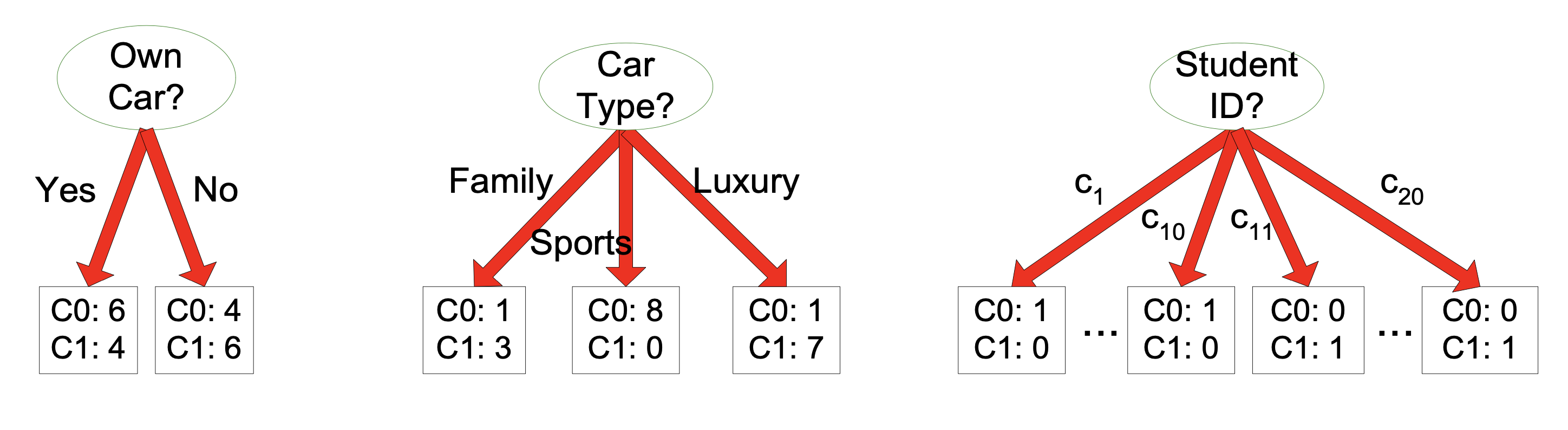
The “Car Type” attribute yields more homogeneous splits.
Using the “Student ID” attribute yields perfect accuracy on the training data.
… but what would it do on the test data?
… using the “Student ID” attribute would lead to overfitting
We’ll talk about how to avoid overfitting shortly.
For now, let’s just focus on maximizing the homogeneity of splits.
We need a measure of homogeneity:
A number of measures have been proposed:
GINI Index
Entropy
Misclassification Error
We will review GINI, as it is a typical measure.
It’s used, for example, in CART, SLIQ, and SPRINT.
Computing GINI#
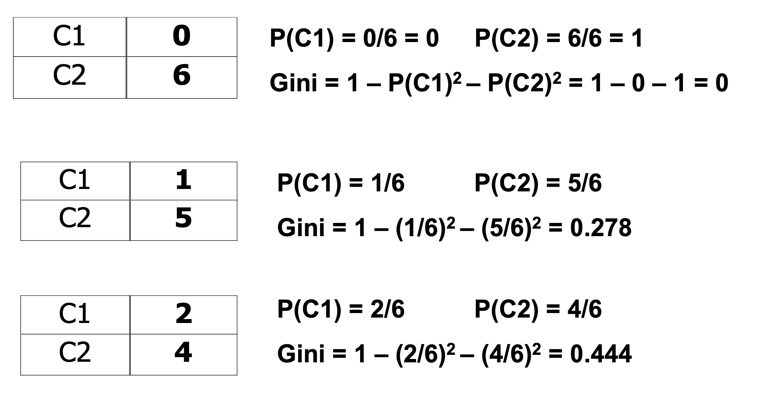
We will think of the set of records at each node as defining a distribution over the classes.
For a given node \(t\), we will use \(p(j\,|\,t)\) to denote the frequency of class \(j\) at node \(t\).
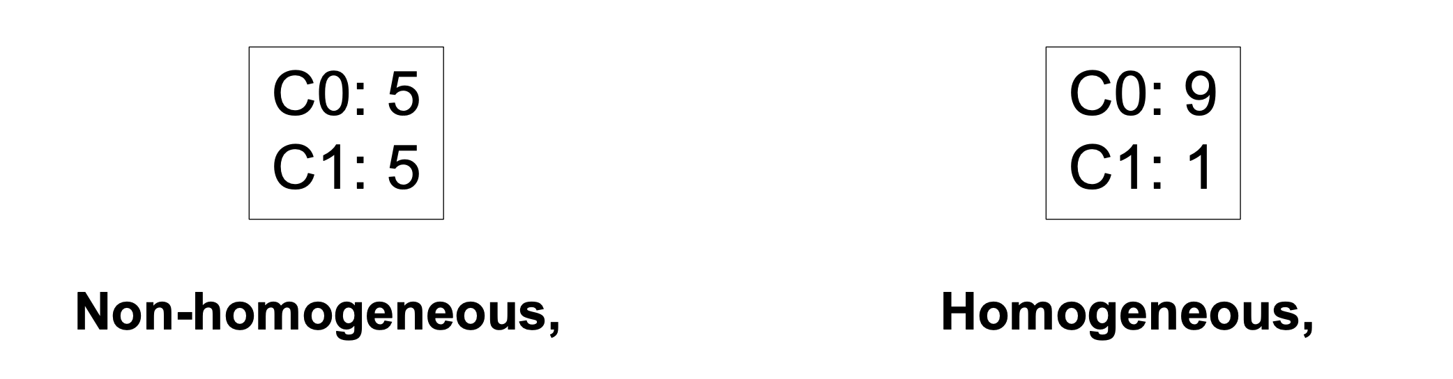
The GINI coefficient measures the degree of “balance” in a distribution.
It is defined as:
As nodes are split in building the tree, we will be decreasing the GINI score.
Now, how do we compute the improvement in GINI when a node is split?
Remember that we would like to create large, homogeneous nodes.
So we will weight each node’s GINI score by the number of records it contains.
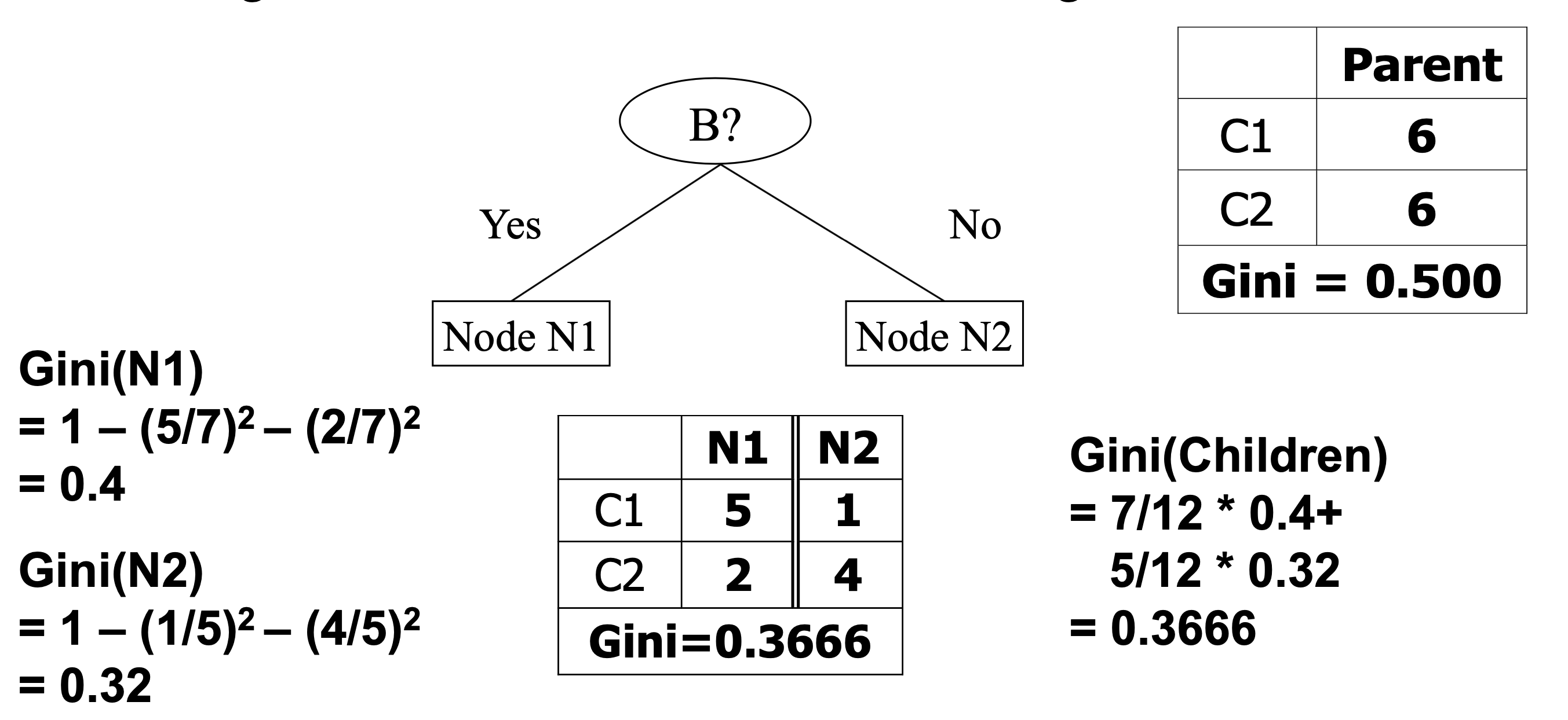
So the improvement in GINI score when splitting a node \(t\) with \(n\) records will be computed as:
where new node \(i\) contains \(n_i\) records;
and the improvement in GINI score will be defined as
GINI for Binary Partitions
Here is an example of computing the new GINI score for a partition:
GINI for Nominal Attributes
For each distinct value, gather counts for each class in the dataset
Use the count matrix to evaluate groupings
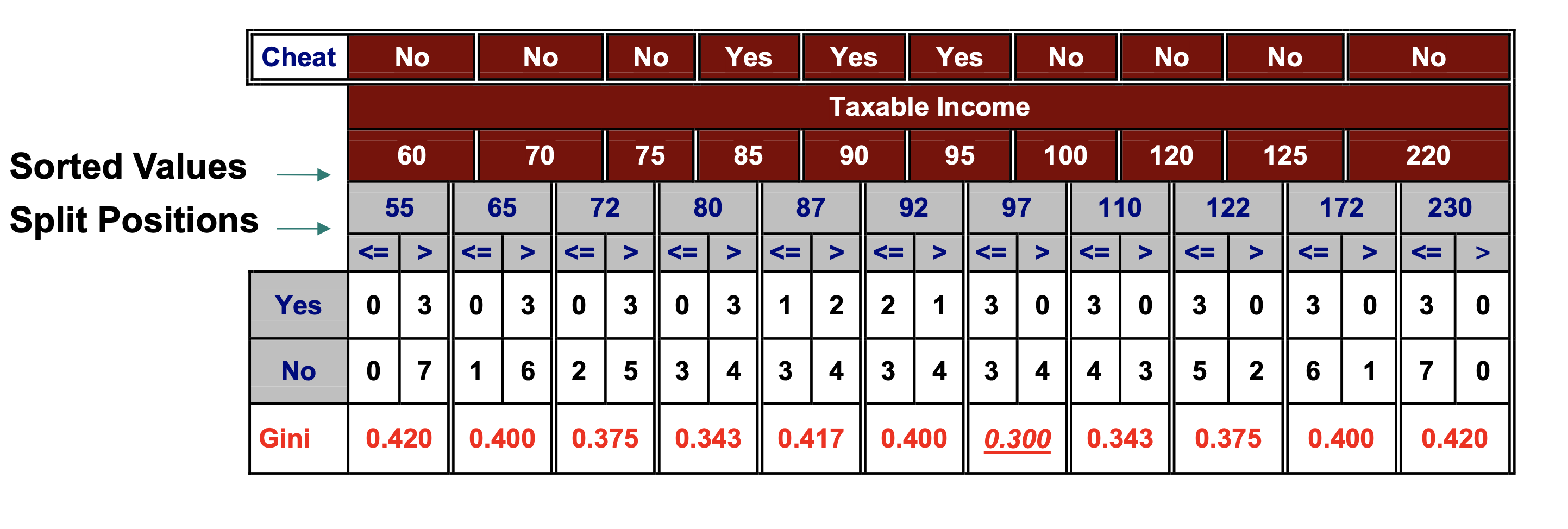
GINI for Continuous Attributes
To find the best threshold efficiently:
Sort the attribute on values
Linearly scan the values,
each time updating a count matrix and
computing the new GINI score
Choose the split position with the smallest GINI index
When to Stop Splitting#
We now see how the decision tree is built, node by node, by splitting nodes in a way that steadily improves the overall GINI score.
Clearly, we could keep on splitting nodes until every leaf node contains only unique training records.
For example, each leaf node could contain just a single training record - a fully-grown tree.
This would certainly be overfitting!
We would have as many leaf nodes (parameters) as training data records.
And we would not expect the decision tree to generalize well.
There are two strategies that can be used to control the complexity of a decision tree:
Early-stopping: stop the algorithm before the tree becomes fully-grown
Post-pruning: grow decision tree fully, then prune nodes from leaves upward
Early Stopping
Do not expand the current node, even though it still has multiple records.
Default stopping conditions include:
Stop if all records belong to the same class
Stop if all the records have the same attributes
More restrictive stopping conditions include:
Stop if number of records in current node is less than a specified value
Stop if expanding the current node does not improve homogeneity (eg, GINI score)
Stop if splitting current node would create node smaller than a specified value
Post-pruning
Assumes that we can assess generalization error
For example, using held-out data
Then:
Grow decision tree to its entirety
Trim the nodes of the tree in bottom-up fashion
Replace nodes with majority class
If generalization error improves after trimming, replace sub-tree by a leaf node
Note that this is computationally more demanding than early-stopping.
Interpretability#
Decision Trees are a very popular technique.
They have a number of advantages:
They are relatively inexpensive to construct
They are extremely fast at classifying unknown data
Their accuracy can be quite good in many cases
And oftentimes they are interpretable
We will explore interpretation of decision trees in a following lecture.