Show code cell content
import numpy as np
import scipy as sp
import matplotlib.pyplot as plt
import pandas as pd
import seaborn as sns
import matplotlib as mp
import sklearn
from IPython.display import Image, HTML
import statsmodels.api as sm
from sklearn import model_selection
from sklearn import metrics

import laUtilities as ut

%matplotlib inline
Logistic Regression#
So far we have seen linear regression: a continuous valued observation is estimated as linear (or affine) function of the independent variables.
Today we will look at the following situation.
Imagine that you are observing a binary variable – a 0/1 value.
That is, these could be pass/fail, admit/reject, Democrat/Republican, etc.
You believe that there is some probability of observing a 1, and that probability is a function of certain independent variables.
So the key properties of a problem that make it appropriate for logistic regression are:
What you can observe is a categorical variable
What you want to estimate is a probability of seeing a particular value of the categorical variable.
What is the probability I will be admitted to Grad School?#
Note
The following example is based on http://www.ats.ucla.edu/stat/r/dae/logit.htm.
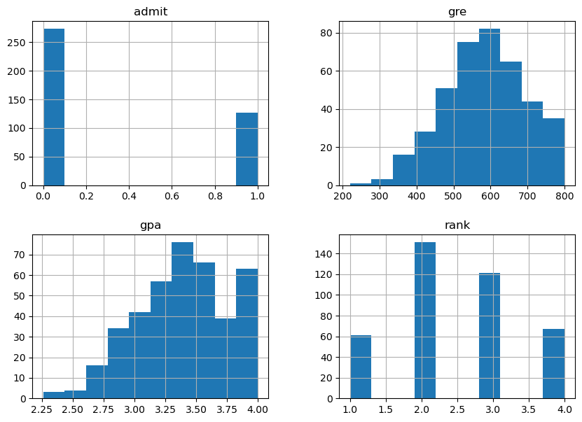
A researcher is interested in how variables, such as GRE (Graduate Record Exam scores), GPA (grade point average) and prestige of the undergraduate institution affect admission into graduate school.
The response variable, admit/don’t admit, is a binary variable.
There are three predictor variables: gre, gpa and rank.
We will treat the variables gre and gpa as continuous.
The variable rank takes on the values 1 through 4.
Institutions with a rank of 1 have the highest prestige, while those with a rank of 4 have the lowest.
# data source: http://www.ats.ucla.edu/stat/data/binary.csv
df = pd.read_csv('data/ats-admissions.csv')
df.head(10)
| admit | gre | gpa | rank | |
|---|---|---|---|---|
| 0 | 0 | 380 | 3.61 | 3 |
| 1 | 1 | 660 | 3.67 | 3 |
| 2 | 1 | 800 | 4.00 | 1 |
| 3 | 1 | 640 | 3.19 | 4 |
| 4 | 0 | 520 | 2.93 | 4 |
| 5 | 1 | 760 | 3.00 | 2 |
| 6 | 1 | 560 | 2.98 | 1 |
| 7 | 0 | 400 | 3.08 | 2 |
| 8 | 1 | 540 | 3.39 | 3 |
| 9 | 0 | 700 | 3.92 | 2 |
df.describe()
| admit | gre | gpa | rank | |
|---|---|---|---|---|
| count | 400.000000 | 400.000000 | 400.000000 | 400.00000 |
| mean | 0.317500 | 587.700000 | 3.389900 | 2.48500 |
| std | 0.466087 | 115.516536 | 0.380567 | 0.94446 |
| min | 0.000000 | 220.000000 | 2.260000 | 1.00000 |
| 25% | 0.000000 | 520.000000 | 3.130000 | 2.00000 |
| 50% | 0.000000 | 580.000000 | 3.395000 | 2.00000 |
| 75% | 1.000000 | 660.000000 | 3.670000 | 3.00000 |
| max | 1.000000 | 800.000000 | 4.000000 | 4.00000 |
Show code cell source
ax = plt.figure(figsize = (10,7)).add_subplot()
df.hist(ax = ax);
/var/folders/nm/m_437v6x2qj7_7k4k5wjbk9r000s6y/T/ipykernel_51130/196177421.py:2: UserWarning: To output multiple subplots, the figure containing the passed axes is being cleared.
  df.hist(ax = ax);
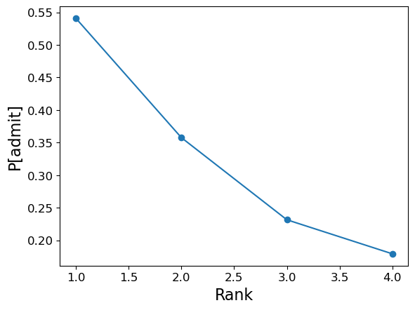
Let’s look at how each independent variable affects admission probability.
First, rank:
Show code cell source
ax = df.groupby('rank').mean()['admit'].plot(marker = 'o',
                                       fontsize = 12)
ax.set_ylabel('P[admit]', fontsize = 16)
ax.set_xlabel('Rank', fontsize = 16);
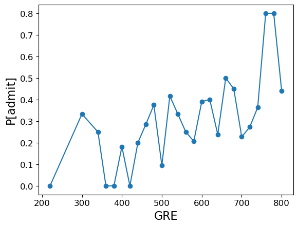
Next, GRE:
Show code cell source
ax = df.groupby('gre').mean()['admit'].plot(marker = 'o',
                                       fontsize = 12)
ax.set_ylabel('P[admit]', fontsize = 16)
ax.set_xlabel('GRE', fontsize = 16);
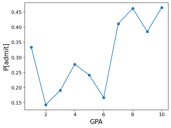
Finally, GPA (for this visualization, we aggregate GPA into 10 bins):
Show code cell source
bins = np.linspace(df.gpa.min(), df.gpa.max(), 10)
ax = df.groupby(np.digitize(df.gpa, bins)).mean()['admit'].plot(marker = 'o',
                                       fontsize = 12)
ax.set_ylabel('P[admit]', fontsize = 16)
ax.set_xlabel('GPA', fontsize = 16);
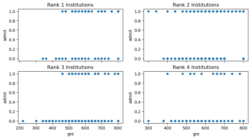
Furthermore, we can see that the independent variables are strongly correlated:
Show code cell source
df1 = df[df['rank']==1]
df2 = df[df['rank']==2]
df3 = df[df['rank']==3]
df4 = df[df['rank']==4]
#
fig = plt.figure(figsize = (10, 5))
ax1 = fig.add_subplot(221)
df1.plot.scatter('gre','admit', ax = ax1)
plt.title('Rank 1 Institutions')
ax2 = fig.add_subplot(222)
df2.plot.scatter('gre','admit', ax = ax2)
plt.title('Rank 2 Institutions')
ax3 = fig.add_subplot(223, sharex = ax1)
df3.plot.scatter('gre','admit', ax = ax3)
plt.title('Rank 3 Institutions')
ax4 = fig.add_subplot(224, sharex = ax2)
plt.title('Rank 4 Institutions')
df4.plot.scatter('gre','admit', ax = ax4);
Logistic Regression#
Logistic regression is concerned with estimating a probability.
However, all that is available are categorical observations, which we will code as 0/1.
That is, these could be pass/fail, admit/reject, Democrat/Republican, etc.
Now, a linear function like \(\alpha + \beta x\) cannot be used to predict probability directly, because the linear function takes on all values (from -\(\infty\) to +\(\infty\)), and probability only ranges over \((0, 1)\).
However, there is a transformation of probability that works: it is called log-odds.
For any probabilty \(p\), the odds is defined as \(p/(1-p)\). Notice that odds vary from 0 to \(\infty\), and odds < 1 indicates that \(p < 1/2\).
Now, there is a good argument that to fit a linear function, instead of using odds, we should use log-odds. That is simply \(\log p/(1-p)\).
Show code cell source
pvec = np.linspace(0.01, 0.99, 100)
ax = plt.figure(figsize = (6, 4)).add_subplot()
ax.plot(pvec, np.log(pvec / (1-pvec)))
ax.tick_params(labelsize=12)
ax.set_xlabel('Probability', fontsize = 14)
ax.set_ylabel('Log-Odds', fontsize = 14)
ax.set_title('Logit Function: $\log (p/1-p)$', fontsize = 16);
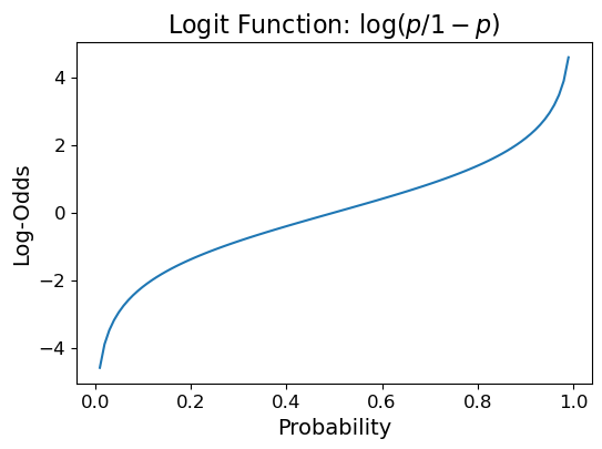
So, logistic regression does the following: it does a linear regression of \(\alpha + \beta x\) against \(\log p/(1-p)\).
That is, it fits:
So, logistic regression fits a probability of the following form: $\(p(x) = P(y=1\mid x) = \frac{e^{\alpha+\beta x}}{1+e^{\alpha+\beta x}}\)$
This is a sigmoid function; when \(\beta > 0\), \(x\rightarrow \infty\), then \(p(x)\rightarrow 1\) and when \(x\rightarrow -\infty\), then \(p(x)\rightarrow 0\).
Show code cell source
alphas = [-4, -8,-12,-20]
betas = [0.4,0.4,0.6,1]
x = np.arange(40)
fig = plt.figure(figsize=(8, 6))
ax = plt.subplot(111)

for i in range(len(alphas)):
    a = alphas[i]
    b = betas[i]
    y = np.exp(a+b*x)/(1+np.exp(a+b*x))
#     plt.plot(x,y,label=r"$\frac{e^{%d + %3.1fx}}{1+e^{%d + %3.1fx}}\;\alpha=%d, \beta=%3.1f$" % (a,b,a,b,a,b))
    ax.plot(x,y,label=r"$\alpha=%d,$    $\beta=%3.1f$" % (a,b))
ax.tick_params(labelsize=12)
ax.set_xlabel('x', fontsize = 14)
ax.set_ylabel('$p(x)$', fontsize = 14)
ax.legend(loc='center left', bbox_to_anchor=(1, 0.5), prop={'size': 16})
ax.set_title('Logistic Functions', fontsize = 16);
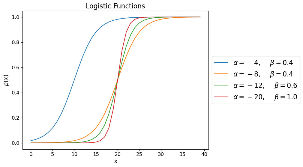
Parameter \(\beta\) controls how fast \(p(x)\) raises from \(0\) to \(1\)
The value of -\(\alpha\)/\(\beta\) shows the value of \(x\) for which \(p(x)=0.5\)
Another interpretation of \(\alpha\) is that it gives the base rate – the unconditional probability of a 1. That is, if you knew nothing about a particular data item, then \(p(x) = 1/(1+e^{-\alpha})\).
The function \(f(x) = \log (x/(1-x))\) is called the logit function.
So a compact way to describe logistic regression is that it finds regression coefficients \(\alpha, \beta\) to fit:
Note also that the inverse logit function is:
Somewhat confusingly, this is called the logistic function.
So, the best way to think of logistic regression is that we compute a linear function:
and then “map” that to a probability using the \(\text{logit}^{-1}\) function:
Logistic vs Linear Regression#
Let’s take a moment to compare linear and logistic regression.
In Linear regression we fit
We do the fitting by minimizing the sum of squared error (\(\Vert\epsilon\Vert\)). This can be done in closed form.
(Recall that the closed form is found by geometric arguments, or by calculus).
Now, if \(\epsilon_i\) comes from a normal distribution with mean zero and some fixed variance,
then minimizing the sum of squared error is exactly the same as finding the maximum likelihood of the data with respect to the probability of the errors.
So, in the case of linear regression, it is a lucky fact that the MLE of \(\alpha\) and \(\beta\) can be found by a closed-form calculation.
In Logistic regression we fit
with \(\text{Pr}(y_i=1\mid x_i)=p(x_i).\)
How should we choose parameters?
Here too, we use Maximum Likelihood Estimation of the parameters.
That is, we choose the parameter values that maximize the likelihood of the data given the model.
We can write this as a single expression:
We then use this to compute the likelihood of parameters \(\alpha\), \(\beta\):
which is a function that we can maximize via various kinds of gradient descent.
Logistic Regression In Practice#
So, in summary, we have:
Input pairs \((x_i,y_i)\)
Output parameters \(\widehat{\alpha}\) and \(\widehat{\beta}\) that maximize the likelihood of the data given these parameters for the logistic regression model.
Method Maximum likelihood estimation, obtained by gradient descent.
The standard package will give us a correlation coefficient (a \(\beta_i\)) for each independent variable (feature).
If we want to include a constant (ie, \(\alpha\)) we need to add a column of 1s (just like in linear regression).
df['intercept'] = 1.0
train_cols = df.columns[1:]
train_cols
Index(['gre', 'gpa', 'rank', 'intercept'], dtype='object')
logit = sm.Logit(df['admit'], df[train_cols])

# fit the model
result = logit.fit()
Optimization terminated successfully.
         Current function value: 0.574302
         Iterations 6
result.summary()
| Dep. Variable: | admit | No. Observations: | 400 |
|---|---|---|---|
| Model: | Logit | Df Residuals: | 396 |
| Method: | MLE | Df Model: | 3 |
| Date: | Wed, 12 Jul 2023 | Pseudo R-squ.: | 0.08107 |
| Time: | 12:43:58 | Log-Likelihood: | -229.72 |
| converged: | True | LL-Null: | -249.99 |
| Covariance Type: | nonrobust | LLR p-value: | 8.207e-09 |
| coef | std err | z | P>|z| | [0.025 | 0.975] | |
|---|---|---|---|---|---|---|
| gre | 0.0023 | 0.001 | 2.101 | 0.036 | 0.000 | 0.004 |
| gpa | 0.7770 | 0.327 | 2.373 | 0.018 | 0.135 | 1.419 |
| rank | -0.5600 | 0.127 | -4.405 | 0.000 | -0.809 | -0.311 |
| intercept | -3.4495 | 1.133 | -3.045 | 0.002 | -5.670 | -1.229 |
Notice that all of our independent variables are considered significant (no confidence intervals contain zero).
Using the Model#
Note that by fitting a model to the data, we can make predictions for inputs that were never seen in the data.
Furthermore, we can make a prediction of a probability for cases where we don’t have enough data to estimate the probability directly – e.g, for specific parameter values.
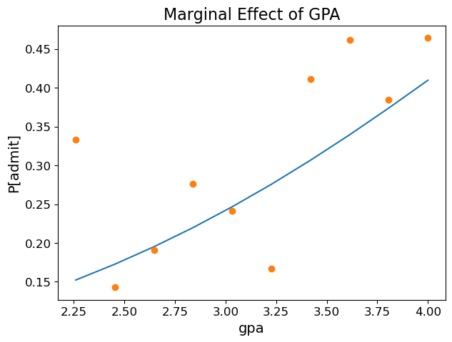
Let’s see how well the model fits the data.
We have three independent variables, so in each case we’ll use average values for the two that we aren’t evaluating.
GPA:
Show code cell source
bins = np.linspace(df.gpa.min(), df.gpa.max(), 10)
groups = df.groupby(np.digitize(df.gpa, bins))
prob = [result.predict([600, b, 2.5, 1.0]) for b in bins]
ax = plt.figure(figsize = (7, 5)).add_subplot()
ax.plot(bins, prob)
ax.plot(bins,groups.admit.mean(),'o')
ax.tick_params(labelsize=12)
ax.set_xlabel('gpa', fontsize = 14)
ax.set_ylabel('P[admit]', fontsize = 14)
ax.set_title('Marginal Effect of GPA', fontsize = 16);
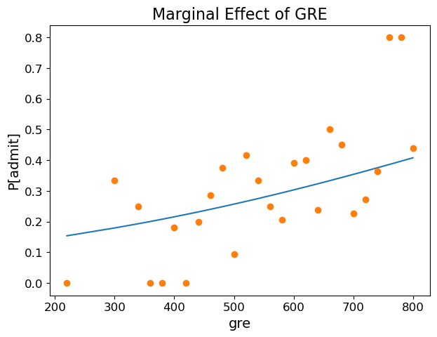
GRE Score:
Show code cell source
prob = [result.predict([b, 3.4, 2.5, 1.0]) for b in sorted(df.gre.unique())]
ax = plt.figure(figsize = (7, 5)).add_subplot()
ax.plot(sorted(df.gre.unique()), prob)
ax.plot(df.groupby('gre').mean()['admit'],'o')
ax.tick_params(labelsize=12)
ax.set_xlabel('gre', fontsize = 14)
ax.set_ylabel('P[admit]', fontsize = 14)
ax.set_title('Marginal Effect of GRE', fontsize = 16);
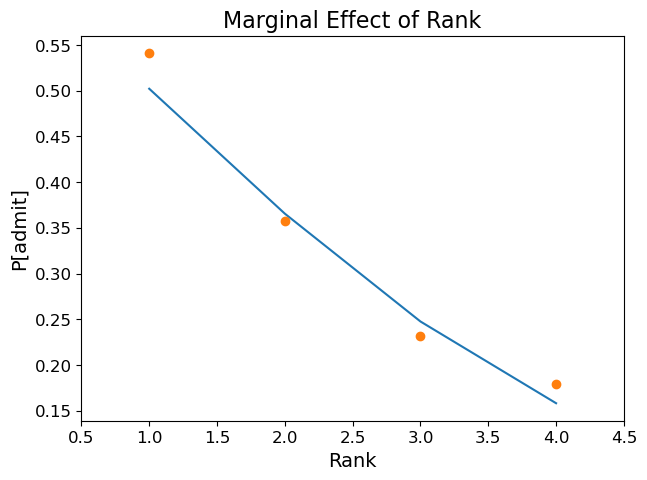
Institution Rank:
Show code cell source
prob = [result.predict([600, 3.4, b, 1.0]) for b in range(1,5)]
ax = plt.figure(figsize = (7, 5)).add_subplot()
ax.plot(range(1,5), prob)
ax.plot(df.groupby('rank').mean()['admit'],'o')
ax.tick_params(labelsize=12)
ax.set_xlabel('Rank', fontsize = 14)
ax.set_xlim([0.5,4.5])
ax.set_ylabel('P[admit]', fontsize = 14)
ax.set_title('Marginal Effect of Rank', fontsize = 16);
Logistic Regression in Perspective#
At the start of lecture I emphasized that logistic regression is concerned with estimating a probability model from discrete (0/1) data.
However, it may well be the case that we want to do something with the probability that amounts to classification.
For example, we may classify data items using a rule such as “Assign item \(x_i\) to Class 1 if \(p(x_i) > 0.5\)”.
For this reason, logistic regression could be considered a classification method.
In fact, that is what we did with Naive Bayes – we used it to estimate something like a probability, and then chose the class with the maximum value to create a classifier.
Let’s use our logistic regression as a classifier.
We want to ask whether we can correctly predict whether a student gets admitted to graduate school.
Let’s separate our training and test data:
X_train, X_test, y_train, y_test = model_selection.train_test_split(
        df[train_cols], df['admit'],
        test_size=0.4, random_state=1)
Now, there are some standard metrics used when evaluating a binary classifier.
Let’s say our classifier is outputting “yes” when it thinks the student will be admitted.
There are four cases:
Classifier says “yes”, and student is admitted: True Positive.
Classifier says “yes”, and student is not admitted: False Positive.
Classifier says “no”, and student is admitted: False Negative.
Classifier says “no”, and student is not admitted: True Negative.
Precision is the fraction of “yes”es that are correct: $\(\mbox{Precision} = \frac{\mbox{True Positives}}{\mbox{True Positives + False Positives}}\)$
Recall is the fraction of admits that we say “yes” to: $\(\mbox{Recall} = \frac{\mbox{True Positives}}{\mbox{True Positives + False Negatives}}\)$
def evaluate(y_train, X_train, y_test, X_test, threshold):

    # learn model on training data
    logit = sm.Logit(y_train, X_train)
    result = logit.fit(disp=False)

    # make probability predictions on test data
    y_pred = result.predict(X_test)

    # threshold probabilities to create classifications
    y_pred = y_pred > threshold

    # report metrics
    precision = metrics.precision_score(y_test, y_pred)
    recall = metrics.recall_score(y_test, y_pred)
    return precision, recall

precision, recall = evaluate(y_train, X_train, y_test, X_test, 0.5)

print(f'Precision: {precision:0.3f}, Recall: {recall:0.3f}')
Precision: 0.586, Recall: 0.340
Now, let’s get a sense of average accuracy:
PR = []
for i in range(20):
    X_train, X_test, y_train, y_test = model_selection.train_test_split(
            df[train_cols], df['admit'],
            test_size=0.4)
    PR.append(evaluate(y_train, X_train, y_test, X_test, 0.5))
avgPrec = np.mean([f[0] for f in PR])
avgRec = np.mean([f[1] for f in PR])
print(f'Average Precision: {avgPrec:0.3f}, Average Recall: {avgRec:0.3f}')
Average Precision: 0.578, Average Recall: 0.215
Sometimes we would like a single value that describes the overall performance of the classifier.
For this, we take the harmonic mean of precision and recall, called F1 Score:
Using this, we can evaluate other settings for the threshold.
import warnings
warnings.filterwarnings("ignore")
def evalThresh(df, thresh):
    PR = []
    for i in range(20):
        X_train, X_test, y_train, y_test = model_selection.train_test_split(
                df[train_cols], df['admit'],
                test_size=0.4)
        PR.append(evaluate(y_train, X_train, y_test, X_test, thresh))
    avgPrec = np.mean([f[0] for f in PR])
    avgRec = np.mean([f[1] for f in PR])
    return 2 * (avgPrec * avgRec) / (avgPrec + avgRec), avgPrec, avgRec

tvals = np.linspace(0.05, 0.8, 50)
f1vals = [evalThresh(df, tval)[0] for tval in tvals]
Show code cell source
plt.plot(tvals,f1vals)
plt.ylabel('F1 Score')
plt.xlabel('Threshold for Classification')
plt.title('F1 as a function of Threshold');
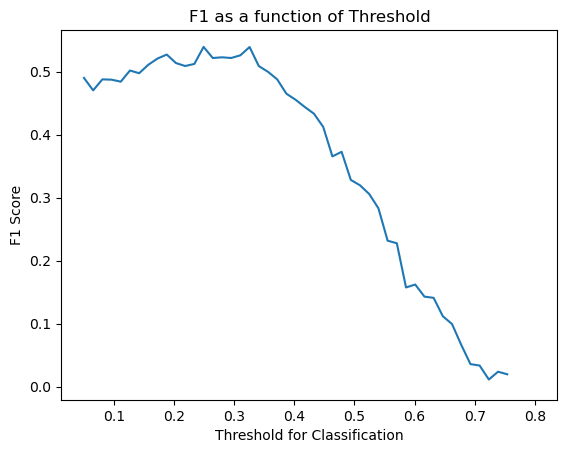
Based on this plot, we can say that the best classification threshold appears to be around 0.3, where precision and recall are:
Show code cell source
F1, Prec, Rec = evalThresh(df, 0.3)
print('Best Precision: {:0.3f}, Best Recall: {:0.3f}'.format(Prec, Rec))
Best Precision: 0.417, Best Recall: 0.677
The example here is based on http://blog.yhathq.com/posts/logistic-regression-and-python.html where you can find additional details.