Gradient Descent

Gradient Descent#

Most of the machine learning we have studied this semester is based on the idea that we have a model that is parameterized, and our goal is to find good settings for the parameters.

We have seen example after example of this problem.

In \(k\)-means, our goal was to find \(k\) cluster centroids, so that the \(k\)-means objective was minimized.
In linear regression, our goal was to find a parameter vector \(\beta\) so that sum of squared error \(\Vert \mathbf{y} - \hat{\mathbf{y}}\Vert\) was minimized.
In the support vector machine, our goal was to find a parameter vector \(\theta\) so that classification error was minimized.

And on and on …

It’s time now to talk about how, in general, one can find “good settings” for the parameters in problems like these.

What allows us to unify our approach to many such problems is the following:

First, we start by defining an error function, generally called a loss function, to describe how well our method is doing.

And second, we choose loss functions that are differentiable with respect to the parameters.

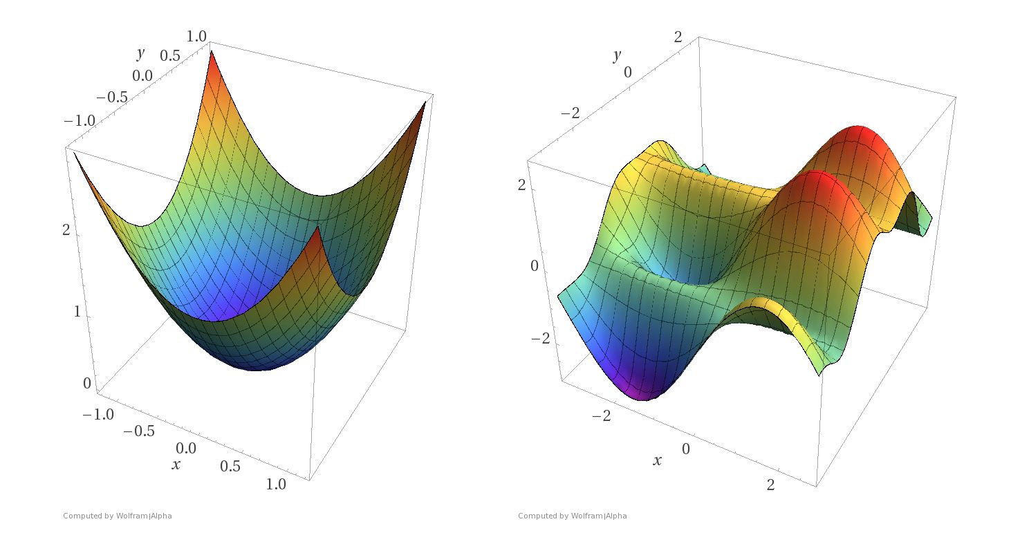
These two requirements mean that we can think of the parameter tuning problem using surfaces like these:

Imagine that the \(x\) and \(y\) axes in these pictures represent parameter settings. That is, we have two parameters to set, corresponding to the values of \(x\) and \(y\).

For each \((x, y)\) setting, the \(z\)-axis shows the value of the loss function.

What we want to do is find the minimum of a surface, corresponding to the parameter settings that minimize loss.

Notice the difference between the two kinds of surfaces.

The surface on the left corresponds to a strictly convex loss function. If we find a local minimum of this function, it is a global minimum.

The surface on the right corresponds to a non-convex loss function. There are local minima that are not globally minimal.

Both kinds of loss functions arise in machine learning.

For example, convex loss functions arise in

Linear regression
Logistic regression

While non-convex loss functions arise in

\(k\)-means
Gaussian Mixture Modeling
and many other settings

Gradient Descent Intuitively#

The intuition of gradient descent is the following.

Imagine you are lost in the mountains, and it is foggy out. You want to find a valley. But since it is foggy, you can only see the local area around you.

The natural thing to do is:

Look around you 360 degrees.
Observe in which direction the ground is sloping downward most steeply.
Take a few steps in that direction.
Repeat the process
… until the ground seems to be level.

Formalizing Gradient Descent#

The key to this intuitive idea is formalizing the idea of “direction of steepest descent.”

This is where the differentiability of the loss function comes into play.

As long as the loss function is differentiable, we can define the direction of steepest descent (really, ascent).

That direction is called the gradient.

The gradient is a generalization of the slope of a line.

Let’s say we have a loss function \(\mathcal{L}(\mathbf{w})\).

The components of \(\mathbf{w}\in\mathbb{R}^n\) are the parameters we want to optimize.

For example, if our problem is linear regression, the loss function could be:

\[ \mathcal{L}(\mathbf{w}) = \Vert\mathbf{y} - \hat{\mathbf{y}}\Vert^2 \]

where \(\hat{\mathbf{y}}\) is our estimate, ie, \(\hat{\mathbf{y}} = X\mathbf{w}\) so that

\[ \mathcal{L}(\mathbf{w}) = \Vert\mathbf{y} - X\mathbf{w}\Vert^2 \]

To find the gradient, we take the partial derivative of our loss function with respect to each parameter:

\[ \frac{\partial \mathcal{L}}{\partial w_i} \]

and collect all the partial derivatives into a vector of the same shape as \(\mathbf{w}\):

\[\begin{split} \nabla_\mathbf{w}\mathcal{L} = \begin{bmatrix} \frac{\partial \mathcal{L}}{\partial w_1}\\ \frac{\partial \mathcal{L}}{\partial w_2}\\ \vdots \\ \frac{\partial \mathcal{L}}{\partial w_n} \end{bmatrix} \end{split}\]

When you see the notation \(\nabla_\mathbf{w}\mathcal{L},\) think of it as \( \frac{d\mathcal{L}}{d\mathbf{w}} \), keeping in mind that \(\mathbf{w}\) is a vector.

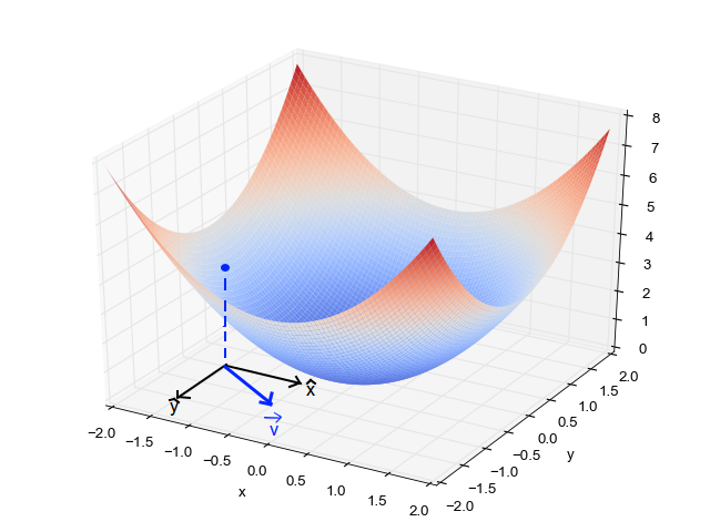
It turns out that if we are going to take a small step of unit length, then the gradient is the direction that maximizes the change in the loss function.

As you can see from the above figure, in general the gradient varies depending on where you are in the parameter space.

So we write:

\[\begin{split} \nabla_\mathbf{w}\mathcal{L}(\mathbf{w}) = \begin{bmatrix} \frac{\partial \mathcal{L}}{\partial w_1}(\mathbf{w})\\ \frac{\partial \mathcal{L}}{\partial w_2}(\mathbf{w})\\ \vdots \\ \frac{\partial \mathcal{L}}{\partial w_n}(\mathbf{w}) \end{bmatrix} \end{split}\]

Each time we seek to improve our parameter estimates \(\mathbf{w}\), we will take a step in the negative direction of the gradient.

… “negative direction” because the gradient specifies the direction of maximum increase – and we want to decrease the loss function.

How big a step should we take?

For step size, will use a scalar value \(\eta\) called the learning rate.

The learning rate is a hyperparameter that needs to be tuned for a given problem, or even can be modified adaptively as the algorithm progresses.

Now we can write the gradient descent algorithm formally:

Start with an initial parameter estimate \(\mathbf{w}^0\).
Update: \(\mathbf{w}^{n+1} = \mathbf{w}^n - \eta \nabla_\mathbf{w}\mathcal{L}(\mathbf{w}^n)\)
If not converged, go to step 2.

How do we know if we are “converged”?

Typically we stop the iteration if the loss has not improved by a fixed amount for a pre-decided number, say 10 or 20, iterations.

Example: Linear Regression#

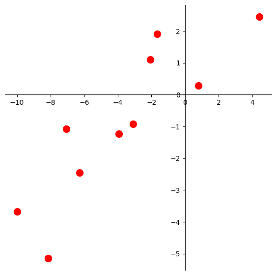
Let’s say we have this dataset.

_images/9581f241ffa7ab5f848e98c2c73a503b64f15229eec527653052a0629d62dd67.png

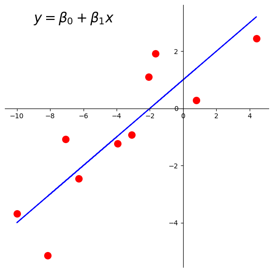
Let’s fit a least-squares line to this data.

The loss function for this problem is the least-squares error:

\[\mathcal{L}(\mathbf{\beta}) = \Vert\mathbf{y} - X\mathbf{\beta}\Vert^2\]

Of course, we know how to solve this problem using the normal equations, but let’s do it using gradient descent instead.

Here is the line we’d like to find:

_images/7107746b2742b2e8b1e542c5742527d2760f3ce622895d2da6ebe17385dfda6e.png

There are \(n = 10\) data points, whose \(x\) and \(y\) values are stored in xlin and y.

First, let’s create our \(X\) (design) matrix, and include a column of ones to model the intercept:

X = np.column_stack([np.ones((n, 1)), xlin])

Now, let’s visualize the loss function \(\mathcal{L}(\mathbf{\beta}) = \Vert \mathbf{y}-X\mathbf{\beta}\Vert^2.\)

_images/4d1ef4ded73c6e40618bff50e2787e54957101b9e1a8e179d2357019f63d231e.png

I won’t take you through computing the gradient for this problem (you can find it in the online text).

I will just tell you that the gradient for a least squares problem is:

\[\nabla_\beta \mathcal{L}(\mathbf{\beta}) = X^T X \beta - X^T\mathbf{y} \]

Note

For those interested in a little more insight into what these plots are showing, here is the derivation.

We start from the rule that \(\Vert \mathbf{v}\Vert = \sqrt{\mathbf{v}^T\mathbf{v}}\).

Applying this rule to our loss function:

\[ \mathcal{L}(\mathbf{\beta}) = \Vert \mathbf{y} - X\mathbf{\beta} \Vert^2 = \beta^T X^T X \beta - 2\mathbf{\beta}^TX^T\mathbf{y} + \mathbf{y}^T\mathbf{y} \]

The first term, \(\beta^T X^T X \beta\), is a quadratic form, and it is what makes this surface curved. As long as \(X\) has independent columns, \(X^TX\) is positive definite, so the overall shape is a paraboloid opening upward, and the surface has a unique minimum point.

To find the gradient, we can use standard calculus rules for derivates involving vectors. The rules are not complicated, but the bottom line is that in this case, you can almost use the same rules you would if \(\beta\) were a scalar:

\[\nabla_\beta \mathcal{L}(\mathbf{\beta}) = 2X^T X \beta - 2X^T\mathbf{y} \]

And by the way – since we’ve computed the derivative as a function of \(\beta\), instead of using gradient descent, we could simply solve for the point where the gradient is zero. This is the optimal point which we know must exist:

\[ \nabla_\beta \mathcal{L}(\mathbf{\beta}) = 0 \]

\[ 2X^T X \beta - 2X^T\mathbf{y} = 0 \]

\[ X^T X \beta = X^T\mathbf{y} \]

Which of course, are the normal equations for this linear system.

So here is our code for gradient descent:

def loss(X, y, beta):
    return np.linalg.norm(y - X @ beta) ** 2

def gradient(X, y, beta):
    return X.T @ X @ beta - X.T @ y

def gradient_descent(X, y, beta_hat, eta, nsteps = 1000):
    losses = [loss(X, y, beta_hat)]
    betas = [beta_hat]
    #
    for step in range(nsteps):
        #
        # the gradient step
        new_beta_hat = beta_hat - eta * gradient(X, y, beta_hat)
        beta_hat = new_beta_hat
        #
        # accumulate statistics
        losses.append(loss(X, y, new_beta_hat))
        betas.append(new_beta_hat)
        
    return np.array(betas), np.array(losses)

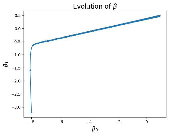
We’ll start at an arbitrary point, say, \((-8, -3.2)\).

That is, \(\beta_0 = -8\), and \(\beta_1 = -3.2\).

beta_start = np.array([-8, -3.2])
eta = 0.002
betas, losses = gradient_descent(X, y, beta_start, eta)

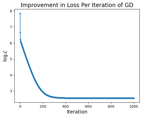
What happens to our loss function per GD iteration?

_images/0de0071b1746dd39d4977252d5560f10fe4eb9ed42e728b5dcf1b27369b746bf.png

_images/eb4dc9a94f7b8472eaeb91148f9e0c41d8e0b8c493ceda06992bfa375e4c1761.png

Notice that the improvement in loss decreases over time. Initially the gradient is steep and loss improves fast, while later on the gradient is shallow and loss doesn’t improve much per step.

Now remember that in reality we are like the person who is trying to find their way down the mountain, in the fog.

In general we cannot “see” the entire loss function surface.

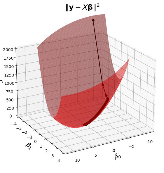
Nonetheless, since we know what the loss surface looks like in this case, we can visualize the algorithm “moving” on that surface.

This visualization combines the last two plots into a single view.

_images/122910d1f40db6c3fbe8378fd17bb7fb236335b6a71da1b9c1bd266e12f8ad93.png

Next we can visualize how the algorithm progresses, both in parameter space and in data space:

Animation size has reached 20999994 bytes, exceeding the limit of 20971520.0. If you're sure you want a larger animation embedded, set the animation.embed_limit rc parameter to a larger value (in MB). This and further frames will be dropped.

Challenges in Gradient Descent#

Gradient Descent is a very general algorithm, one that can be applied to a huge array of problem types.

However, there are a variety of issues that arise in using gradient descent in practice.

Learning Rate#

Setting the learning rate can be a challenge.

Previously we had set the learning rate \(\eta = 0.002\).

Let set it a little higher and see what happens: \(\eta = 0.0065.\)

beta_start = np.array([-8, -2])
eta = 0.0065
betas, losses = gradient_descent(X, y, beta_start, eta, nsteps = 100)

_images/f5b24f0e144afb8abcbccc4770763747d6eb02e0a1509a9e324402cec31c8e47.png

_images/e9d9fe22d2d51f3da444c1e30ad7a71a3e673da54a98eb11b4d83fac91b3ee8d.png

This is a total disaster. What is going on?

It is helpful to look at the progress of the algorithm using the loss surface:

_images/d2877e015a54d3be41bd84b73190e7bcdd720e264c279413ffe363b60a5f8a0b.png

We can see what is going on more clearly here.

What is happening is that because the steps are too large, each step overshoots the local minimum.

The next step then lands on a portion of the surface that steeper … and in the opposite direction.

And so the process diverges.

Note

For an interesting comparison, try setting \(\eta = 0.0055\) and observe the evolution of \(\beta\).

Hence it is important to decrease the step size when divergence appears.

Unfortunately, on a complicated loss surface, a given step size may diverge in one location or starting point, but not in another.

Complex Loss Surfaces#

The loss surface for linear regression is the best possible kind: it is strictly convex, so it has a single global minimum.

For many problems, the loss surface is more complex.

In particular, the more complex the model, the more complex the loss surface.

The most complex models in use today are deep neural nets, some of which have billions of parameters.

For example, here is a visualization of the loss surface for a deep neural net:

Depending on the starting values of the parameters, gradient descent can get trapped in a local minimum on a surface like this.

Furthermore, the varying magnitude of the gradient in different regions of this surface creates significant convergence challenges.

Efficiency#

There are two ways in which gradient descent can be slow:

the number of steps taken
the time taken in each step

We have discussed how setting the learning rate \(\eta\) can affect the number of steps taken.

The time taken in each step depends on the cost of computing the gradient.

To understand the issue here, let’s look at the gradient computation more closely.

Assume that the model is denoted \(\hat{y} = f(\mathbf{x}; \mathbf{w}).\)

That is, any prediction is based on inputs \(\mathbf{x}\) and uses parameters \(\mathbf{w}\).

The most common loss function is the sum of squared error:

\[ \mathcal{L}(\mathbf{w}) = \sum_i (\hat{y}_i - y_i)^2 \]

So

\[ \mathcal{L}(\mathbf{w}) = \sum_i (f(\mathbf{x}_i; \mathbf{w}) - y_i)^2 \]

Now note that the gradient operator is a linear operator. In other words:

\[ \nabla_\mathbf{w}\mathcal{L}(\mathbf{w}) = \nabla_\mathbf{w} \sum_i \left[(f(\mathbf{x}_i; \mathbf{w}) - y_i)^2\right] \]

\[ = \sum_i \nabla_\mathbf{w}\left[(f(\mathbf{x}_i; \mathbf{w}) - y_i)^2\right] \]

So the gradient is a sum of terms, each of which is the gradient with respect to a single data item.

Just using the rules of calculus, we can go even further:

\[ \nabla_\mathbf{w}\mathcal{L}(\mathbf{w}) = \sum_i 2 \cdot (f(\mathbf{x}_i; \mathbf{w}) - y_i) \cdot \nabla_\mathbf{w}f(\mathbf{x}_i; \mathbf{w})\]

We can interpret this intuitively:

\[ \nabla_\mathbf{w}\mathcal{L}(\mathbf{w}) = \sum_i 2 \cdot \underbrace{(f(\mathbf{x}_i; \mathbf{w}) - y_i)}_\text{size, sign of error}\;\cdot\underbrace{\nabla_\mathbf{w}f(\mathbf{x}_i; \mathbf{w})}_\text{dir. of prediction increase}\]

Now, with this formulation in mind, we can introduce the most common form of gradient descent: stochastic gradient descent.

Stochastic Gradient Descent#

In modern big data problems, evaluating the gradient over all the (billions) of data points can be expensive.

Often it turns out that a good estimate of the gradient can be computed from a subset of the data.

In the extreme case, we could compute the gradient of a single data point.

Let’s see what that looks like for linear regression.

\[ \nabla_\mathbf{w}\mathcal{L}(\mathbf{w}) = \sum_i 2 \cdot (\mathbf{x}_i^T\beta - y_i) \cdot \nabla_\mathbf{\beta} \mathbf{x}_i^T\beta\]

Again, the rules of calculus for vectors are similar to scalars.

Similar to \(\frac{d}{dx} ax = a\), we find \(\nabla_\mathbf{\beta} \mathbf{x}_i^T\beta = \mathbf{x}_i.\)

So:

\[ \nabla_\mathbf{w}\mathcal{L}(\mathbf{w}) = \sum_i 2 \cdot (\mathbf{x}_i^T\beta - y_i) \cdot \mathbf{x}_i\]

So for linear regression, the loss gradient with respect to a single data point is:

\[ (\mathbf{x}_i^T\beta - y_i) \cdot \mathbf{x}_i \]

The idea of stochastic gradient descent is,

instead of computing the gradient based on all the data,
compute it based on a single data point.

Then repeat the above, iterating over every data point.

So the algorithm for stochastic gradient descent for a dataset of \(n\) points is:

Start with an initial parameter estimate \(\mathbf{w}^0\).
for i = 1 to \(n\):
1. Update: \(\mathbf{w}^{m+1} = \mathbf{w}^m - \eta \cdot (f(\mathbf{x}_i; \mathbf{w}^m) - y_i) \cdot \nabla_\mathbf{w}f(\mathbf{x}_i; \mathbf{w}^m)\)
If not converged, go to step 2.

def loss(X, y, beta):
    return np.linalg.norm(y - X @ beta) ** 2

def point_gradient(x, y, beta):
    return (x.T @ beta - y) * x

def stochastic_gradient_descent(X, y, beta_hat, eta, nsteps = 1000):
    losses = [loss(X, y, beta_hat)]
    betas = [beta_hat]
    #
    for step in range(nsteps):
        #
        for i in range(X.shape[0]):
            #
            # the gradient step
            new_beta_hat = beta_hat - eta * point_gradient(X[i], y[i], beta_hat)
            beta_hat = new_beta_hat
            #
            # accumulate statistics
            losses.append(loss(X, y, new_beta_hat))
            betas.append(new_beta_hat)
        
    return np.array(betas), np.array(losses)

Let’s see how well this works in practice:

beta_start = np.array([-8, -3.2])
eta = 0.002
betas, losses = stochastic_gradient_descent(X, y, beta_start, eta, nsteps = 400)

_images/21fca18e2c4465fa75324ca8255e3ab354ec4d775007d5941fac6d2e1fa97324.png

_images/b94bcfb0f79ecfcdd4786e2e0922111be7e7d2581536f6bd0a01769b6cade320.png

In these plots, each plot point corresponds to an update based on a single data point.

Clearly, the progress is more erratic; we are not taking the most efficent path possible.

We can see in the evolution of \(\beta\) that we don’t go exactly in the correct direction, but close enough that we eventually get to the correct solution.

And each step only requires 1/\(n\) times as much computation as the full gradient!

_images/820038b746068a1339a593c9999868917b1f5eeee75b76a6c67321dd2ec33fc8.png

Different Loss Functions: Logistic Regression#

Finally, we’ll take a look at using different loss functions. For that purpose we’ll return to logistic regression from earlier in the course.

In the linear regression problem, we started with the definition of the loss function:

\[ \mathcal{L}(\mathbf{w}) = \sum_i (\hat{y}_i - y_i)^2 \]

As we’ve mentioned in the past, the most natural approach to classification problems is via probability. How should we think about loss in that case?

We will see that much of what we’ve done already applies nonetheless.

A typical example of a probabilistic classifier is logistic regression.

Recall that the goal of logistic regression is to maximize the likelihood of the data given the model.

To simply notation we will define the logistic function

\[\sigma(t) = \frac{1}{1+e^{-t}} \]

This is the “squashing” function that maps the entire real line \([-\infty, \infty]\) into \([0, 1]\) so the result can be interpreted as a probability.

We then say that \(p(y = 1 \mid x) = \sigma(\alpha + \beta x)\)

For a single data point, the likelihood function for logistic regression is:

\[L(\alpha, \beta \mid x_i, y_i) = \sigma(\alpha + \beta x_i)^{y_i} (1-\sigma(\alpha + \beta x_i))^{1-y_i}\]

And for multiple data points, we multiply the probabilities of the individual data points:

\[L(\alpha, \beta) = \prod_i \sigma(\alpha + \beta x_i)^{y_i} (1-\sigma(\alpha + \beta x_i))^{1-y_i}\]

We’d like to maximize the likelihood. We’ll take the log of it for convenience.

\[\log L(\alpha, \beta) = \sum_i \log(\sigma(\alpha + \beta x_i)^{y_i} (1-\sigma(\alpha + \beta x_i))^{1-y_i})\]

\[= \sum_i y_i \log(\sigma(\alpha + \beta x_i))+ (1-y_i) \log(1-\sigma(\alpha + \beta x_i))\]

To create a loss function that we can minimize, we negate the log likelihood.

Negative log likelihood is called cross entropy loss.

\[\mathcal{L}(\alpha, \beta) = - \sum_i y_i \log(\sigma(\alpha + \beta x_i))+ (1-y_i) \log(1-\sigma(\alpha + \beta x_i))\]

Let’s denote \(\theta = [\alpha, \beta]^T\) and \(\mathbf{x}_i = [1, x_i]^T\). In this notation:

\[\mathcal{L}(\mathbf{\theta}) = - \sum_i y_i \log(\sigma(\theta^T\mathbf{x}_i))+ (1-y_i) \log(1-\sigma(\theta^T\mathbf{x}_i))\]

Then it is a relatively straightforward application of calculus (see the online notes) to show that

\[\nabla_\theta\mathcal{L} = \sum_i (\sigma(\theta^T\mathbf{x}_i) - y_i) \mathbf{x}_i \]

Note

To take the gradient, the key is to use calculus to notice that \(\frac{d}{dt}\sigma(t) = \sigma(t)(1-\sigma(t))\). Using this fact, we can then find that \(\frac{d}{d\mathbf{\theta}} [y_i \log(\sigma(\theta^T\mathbf{x}_i)) + (1-y_i) \log(1-\sigma(\theta^T\mathbf{x}_i))] = (\sigma(\theta^T\mathbf{x}_i)- y_i) \mathbf{x}_i.\)

OK, let’s see how this applies to a problem.

Here is a typical sort of logistic regression problem (in fact, I took it from Wikipedia!):

A group of 20 students spends between 0 and 6 hours studying for an exam. How does the number of hours spent studying affect the probability of the student passing the exam?

_images/0bc0fc5540e036be1c6fe87ae198e8a1f9a1211952da7b2111a9c588ec750e2b.png

Let’s write down our loss and gradient functions.

Note that we don’t need to write a new gradient descent function – we will just provide a new gradient function.

X = np.column_stack([np.ones((len(x), 1)), x])

def sigmoid(x):
    return 1 / (1 + np.exp(-x))

def loss(X, y, theta):
    s = sigmoid(X @ theta)
    return - np.sum(np.array([yi * np.log(si) + (1-yi) * np.log(1-si) for yi, si in zip(y, s)]))

def gradient(X, y, theta):
    return np.sum(np.diag(sigmoid(X @ theta) - y) @ X, axis = 0)

theta_start = np.array([1, 1])
eta = 0.01
thetas, losses = gradient_descent(X, y, theta_start, eta)

Unfortunately we no longer have a closed form expression for the loss surface.

Still, we can observe how the loss declines per iteration:

_images/46a76dbfb260f4914e8123f3221e3449637945bc564dadb7f7ee5f77da191acf.png

And we can see how the parameters evolve, from four different starting points:

_images/cea8a6eb35cf5891460eb4aec5de3ceeb2d341e81bb514710c95ed22eef0ae07.png

And finally we can observe how the logistic function reaches its optimal setting as gradient descent progresses:

Gradient Descent

Contents

Gradient Descent#

Gradient Descent Intuitively#

Formalizing Gradient Descent#

Example: Linear Regression#

Challenges in Gradient Descent#

Learning Rate#

Complex Loss Surfaces#

Efficiency#

Stochastic Gradient Descent#

Different Loss Functions: Logistic Regression#