NN III – Stochastic Gradient Descent, Batches and Convolutional Neural Networks
Contents
NN III – Stochastic Gradient Descent, Batches and Convolutional Neural Networks#
Recap#
So far we covered
Gradients, gradient descent and back propagation
Fully connected neural networks (Multi-Layer Perceptron)
Training of MLPs using back propagation
Today, we’ll cover
Stochastic gradient descent (SGD)
Convolutional Neural Networks (CNNs)
Training a CNN with SGD
Batches and Stochastic Gradient Descent#
Compute the gradient (e.g. forward pass and backward pass) with only a random subset of the input data.
We call the subset a batch.
Work through the dataset by randomly sampling without replacement. This is the stochastic part.
One pass through the data is called an epoch.
For squared error loss with \(N\) input samples, the loss for (full-batch) gradient descent was
For Stochastic Gradient Descent, we calculate the loss only on a batch at as time. For every time \(t\), let’s denote the batch as \(\mathcal{B}_t\)
Let’s look at an example.
import numpy as np
import matplotlib.pyplot as plt

# Generate 12 evenly spaced x values between 1 and 4
x = np.linspace(1, 4, 12)

# Add normally distributed noise to the x values
x += np.random.normal(0, 1.0, 12)

# Calculate the corresponding y values for the line y = 2x
y = 2 * x

# Add normally distributed noise to the y values
y += np.random.normal(0, 1.0, 12)

# Shuffle the points and split them into 3 groups of 4
indices = np.random.permutation(12)
colors = ['red', 'green', 'blue', 'purple']
labels = ['batch 1', 'batch 2', 'batch 3', 'batch 4']

# Plot each group of points with a different color and label
for i in range(4):
    plt.scatter(x[indices[i*3:(i+1)*3]], y[indices[i*3:(i+1)*3]], color=colors[i], label=labels[i])

# Display the legend
plt.legend()

plt.show()
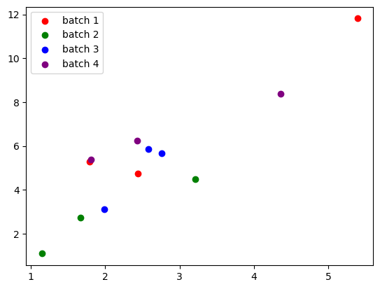
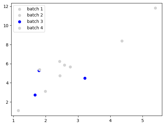
Say we have a training data set of 12 points and we want to use a batch size of 3.
Divide the 12 points into batches of 3 by randomlly selecting points without replacement.
# Shuffle the points and split them into 3 groups of 4
indices = np.random.permutation(12)
colors = ['red', 'green', 'blue', 'purple']
labels = ['batch 1', 'batch 2', 'batch 3', 'batch 4']

# Plot each group of points with a different color and label
for i in range(4):
    plt.scatter(x[indices[i*3:(i+1)*3]], y[indices[i*3:(i+1)*3]], color=colors[i], label=labels[i])

# Display the legend
plt.legend()

plt.show()
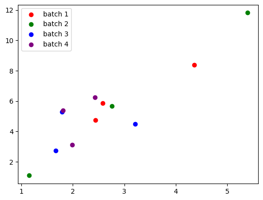
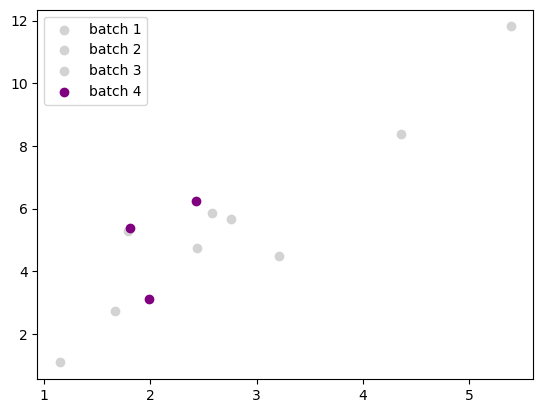
We can resample again to create a different set of batches.
Optionally, you can shuffle after every epoch.
colors = ['red', 'lightgray', 'lightgray', 'lightgray']
labels = ['batch 1', 'batch 2', 'batch 3', 'batch 4']

# Plot each group of points with a different color and label
for i in range(4):
    plt.scatter(x[indices[i*3:(i+1)*3]], y[indices[i*3:(i+1)*3]], color=colors[i], label=labels[i])

# Display the legend
plt.legend()

plt.show()
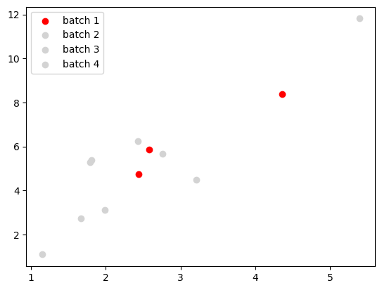
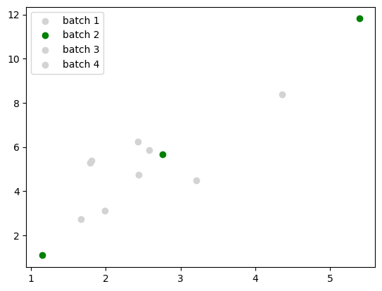
Then for every training iteration, you calculate the forward pass and backward pass loss with only the data from the batch.
Above, we use data from the 1st batch.
colors = ['lightgray', 'green', 'lightgray', 'lightgray']
labels = ['batch 1', 'batch 2', 'batch 3', 'batch 4']

# Plot each group of points with a different color and label
for i in range(4):
    plt.scatter(x[indices[i*3:(i+1)*3]], y[indices[i*3:(i+1)*3]], color=colors[i], label=labels[i])

# Display the legend
plt.legend()

plt.show()
colors = ['lightgray', 'lightgray', 'blue', 'lightgray']
labels = ['batch 1', 'batch 2', 'batch 3', 'batch 4']

# Plot each group of points with a different color and label
for i in range(4):
    plt.scatter(x[indices[i*3:(i+1)*3]], y[indices[i*3:(i+1)*3]], color=colors[i], label=labels[i])

# Display the legend
plt.legend()

plt.show()
colors = ['lightgray', 'lightgray', 'lightgray', 'purple']
labels = ['batch 1', 'batch 2', 'batch 3', 'batch 4']

# Plot each group of points with a different color and label
for i in range(4):
    plt.scatter(x[indices[i*3:(i+1)*3]], y[indices[i*3:(i+1)*3]], color=colors[i], label=labels[i])

# Display the legend
plt.legend()

plt.show()
Advantages of Stochastic Gradient Descent#
There are two main advantages to Stochastic Gradient Descent.
You don’t read and compute on every input data sample for every training iteration,
Speeds up iteration while still making optimization progress
This works better with limited GPU memory and CPU cache. Not slowing down by thrashing limited memory.
Improves training convergence by adding noise to the weight updates.
Can avoid getting stuck in a local minima.
An example

This a contour plot showing a loss surface for a model with only 2 parameters.
For full-batch gradient descent, starting points 1 and 3 still end up at the global minimum, but starting point 2 get stuck in a local minimum.
For stochastic gradient descent, starting point 1 still ends up at the global minimum, but now starting point 2 also avoids the local minimum and ends up at the global minimum.
Load an Image Dataset in Batches in PyTorch#
%matplotlib inline
import torch
import torchvision
import torchvision.transforms as transforms
1. Load and Scale MNIST#
Load MNIST handwritten digit dataset with 60K training samples and 10K test samples.
# Define a transform to scale the pixel values from [0, 255] to [-1, 1]
transform = transforms.Compose([transforms.ToTensor(),
                                transforms.Normalize((0.5,), (0.5,))])

batch_size = 64

# Download and load the training data
trainset = torchvision.datasets.MNIST('./data/MNIST_data/', download=True,
                                    train=True, transform=transform)
trainloader = torch.utils.data.DataLoader(trainset, batch_size=batch_size,
                                          shuffle=True)

# Download and load the test data
testset = torchvision.datasets.MNIST('./data/MNIST_data/', download=True,
                                    train=False, transform=transform)
testloader = torch.utils.data.DataLoader(testset, batch_size=batch_size,
                                         shuffle=True)
Downloading http://yann.lecun.com/exdb/mnist/train-images-idx3-ubyte.gz
Downloading http://yann.lecun.com/exdb/mnist/train-images-idx3-ubyte.gz to ./data/MNIST_data/MNIST/raw/train-images-idx3-ubyte.gz
100%|███████████████████████████| 9912422/9912422 [00:00<00:00, 63641975.04it/s]
Extracting ./data/MNIST_data/MNIST/raw/train-images-idx3-ubyte.gz to ./data/MNIST_data/MNIST/raw

Downloading http://yann.lecun.com/exdb/mnist/train-labels-idx1-ubyte.gz
Downloading http://yann.lecun.com/exdb/mnist/train-labels-idx1-ubyte.gz to ./data/MNIST_data/MNIST/raw/train-labels-idx1-ubyte.gz
100%|███████████████████████████████| 28881/28881 [00:00<00:00, 46501226.04it/s]
Extracting ./data/MNIST_data/MNIST/raw/train-labels-idx1-ubyte.gz to ./data/MNIST_data/MNIST/raw

Downloading http://yann.lecun.com/exdb/mnist/t10k-images-idx3-ubyte.gz
Downloading http://yann.lecun.com/exdb/mnist/t10k-images-idx3-ubyte.gz to ./data/MNIST_data/MNIST/raw/t10k-images-idx3-ubyte.gz
100%|███████████████████████████| 1648877/1648877 [00:00<00:00, 28857335.86it/s]
Extracting ./data/MNIST_data/MNIST/raw/t10k-images-idx3-ubyte.gz to ./data/MNIST_data/MNIST/raw

Downloading http://yann.lecun.com/exdb/mnist/t10k-labels-idx1-ubyte.gz
Downloading http://yann.lecun.com/exdb/mnist/t10k-labels-idx1-ubyte.gz to ./data/MNIST_data/MNIST/raw/t10k-labels-idx1-ubyte.gz
100%|██████████████████████████████████| 4542/4542 [00:00<00:00, 4837615.23it/s]
Extracting ./data/MNIST_data/MNIST/raw/t10k-labels-idx1-ubyte.gz to ./data/MNIST_data/MNIST/raw
torchvision.dataset.MNIST is a convenience class which inherits from
torch.utils.data.Dataset (see doc)
that wraps a particular dataset and overwrites a __getitem__() method which retrieves a data sample given an
index or a key.
If we give the argument train=True, it returns the training set, while the
argument train=False returns the test set.
torch.utils.data.DataLoader() takes a dataset as in the previous line and
returns a python iterable which lets you loop through the data.
We give DataLoader the batch size, and it will return a batch of data samples
on each iteration.
By passing shuffle=True, we are telling the data loader to shuffle the batches
after every epoch.
print(f"No. of training images: {len(trainset)}")
print(f"No. of test images: {len(testset)}")
print("The dataset classes are:")
print(trainset.classes)
No. of training images: 60000
No. of test images: 10000
The dataset classes are:
['0 - zero', '1 - one', '2 - two', '3 - three', '4 - four', '5 - five', '6 - six', '7 - seven', '8 - eight', '9 - nine']
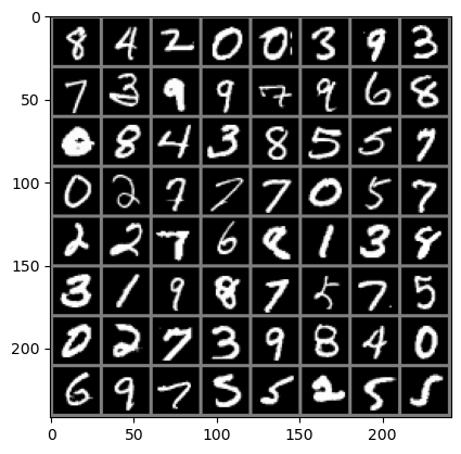
We can see the data loader, trainloader in action in the code below to
get a batch and visualize it.
Everytime we rerun the cell we will get a different batch.
import matplotlib.pyplot as plt
import numpy as np

def imshow(img):
    img = img / 2 + 0.5     # unnormalize
    npimg = img.numpy()
    plt.imshow(np.transpose(npimg, (1, 2, 0)))
    plt.show()

# get some random training images
dataiter = iter(trainloader)
images, labels = next(dataiter)

# show images
imshow(torchvision.utils.make_grid(images))
We can display the training labels for the image as well.
from IPython.display import display, HTML

# Assuming batch_size is 64 and images are displayed in an 8x8 grid
labels_grid = [trainset.classes[labels[j]] for j in range(64)]
labels_grid = np.array(labels_grid).reshape(8, 8)

df = pd.DataFrame(labels_grid)

# Generate HTML representation of DataFrame with border
html = df.to_html(border=1)

# Display the DataFrame
display(HTML(html))
| 0 | 1 | 2 | 3 | 4 | 5 | 6 | 7 | |
|---|---|---|---|---|---|---|---|---|
| 0 | 8 - eight | 4 - four | 2 - two | 0 - zero | 0 - zero | 3 - three | 9 - nine | 3 - three |
| 1 | 7 - seven | 3 - three | 9 - nine | 9 - nine | 7 - seven | 9 - nine | 6 - six | 8 - eight |
| 2 | 0 - zero | 8 - eight | 4 - four | 3 - three | 8 - eight | 5 - five | 5 - five | 7 - seven |
| 3 | 0 - zero | 2 - two | 7 - seven | 7 - seven | 7 - seven | 0 - zero | 5 - five | 7 - seven |
| 4 | 2 - two | 2 - two | 7 - seven | 6 - six | 8 - eight | 1 - one | 3 - three | 8 - eight |
| 5 | 3 - three | 1 - one | 9 - nine | 8 - eight | 7 - seven | 5 - five | 7 - seven | 5 - five |
| 6 | 0 - zero | 2 - two | 7 - seven | 3 - three | 9 - nine | 8 - eight | 4 - four | 0 - zero |
| 7 | 6 - six | 9 - nine | 7 - seven | 5 - five | 5 - five | 2 - two | 5 - five | 5 - five |
Convolutional Network Applications#

Multi-class classification problem ( >2 possible classes)
Convolutional network with classification output
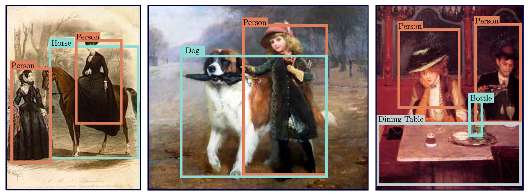
Localize and classify objects in an image
Convolutional network with classification and regression output
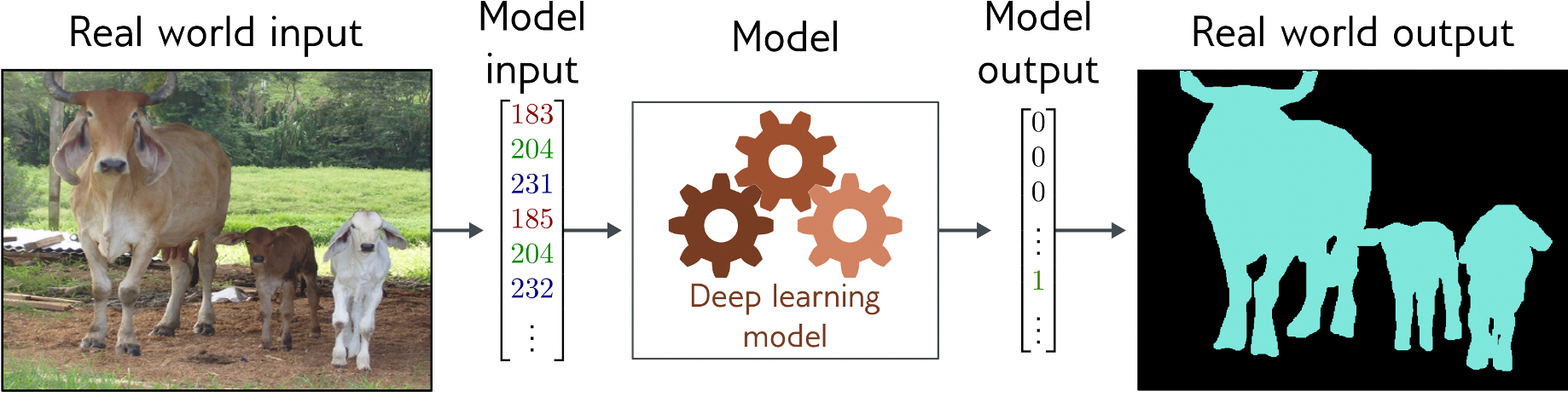
Classify each pixel in an image to 2 or more classes
Convolutional encoder-decoder network with a classification values for each pixel.
Convolutional Neural Networks#
Problems with fully-connected networks
Size
224x224 RGB image = 150,528 dimensions
Hidden layers generally larger than inputs
One hidden layer = 150,520x150,528 weights – 22 billion
Nearby pixels statistically related
But fully connected network doesn’t exploit spatial correlation
Should be stable under transformations
Don’t want to re-learn appearance at different parts of image
Classification Invariant to Shift#
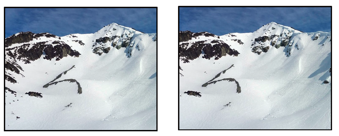
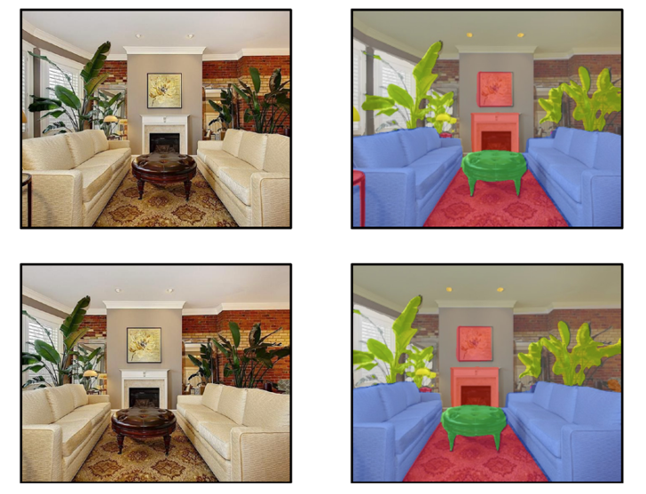
Image Segmentation Invariant to Shift#
Solution: Convolutional Neural Networks
Parameters only look at local data regions
Shares parameters across image or signal
Example with 1-D Input Data#
In convolutional neural networks, we define a set of weights that we move across the input data.
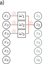
Example with 3 weights and input of length 6.
For figure (a), we calculate
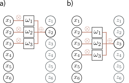
To calculate \(z_2\), we shift the weights over 1 place (figure (b)) and then weight and sum the inputs. We can generalize the equation slightly.
But what do we do about \(z_1\)?
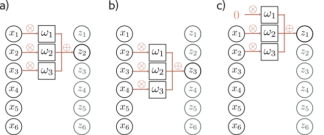
We can calculate \(z_1\) by padding our input data. In figure (c), we simply add \(0\), which means we can now calculate \(z_1\).
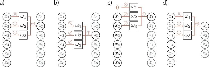
Alternatively, we can just reduce the size of the output, by only calculating where we have valid input data, as in figure (d).
For 1-D data, this reduces the output size by 1 at the beginning and end of the data, so by 2 overall for length-3 filter.
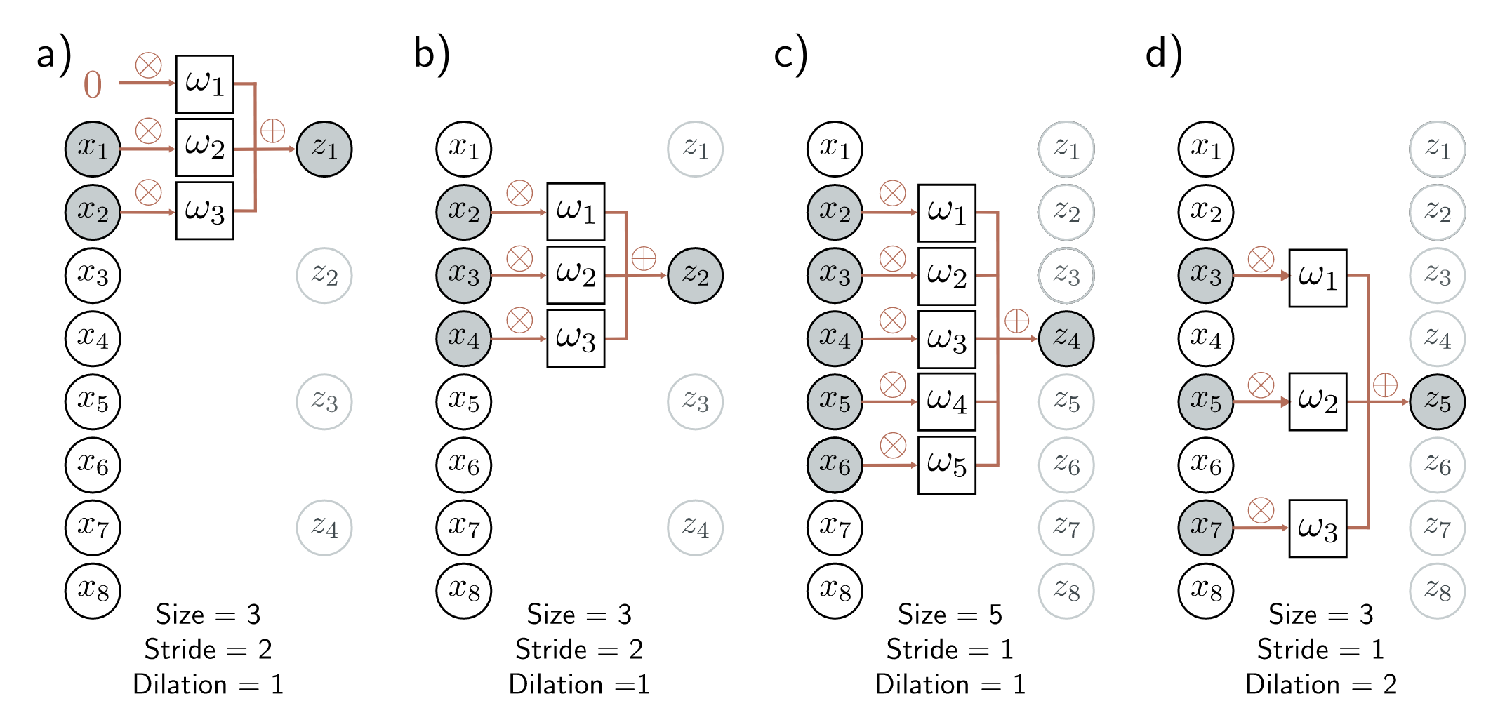
There are a few design choices one can make with convolution layers, such as:
filter length, e.g. size 3 in figures (a) and (b)
stride, which is how much you shift to calculate the next output. Common values are
stride 1 as we saw in the previous examples and in figures (c) and (d)
stride 2, where you shift by 2 instead of 1, an effectively halve the size of the output as in figures (a) and (b)
dilation, where you expand the filter as in figure (d)
2D Convolution#
For images and video frames we use a two-dimensional convolution
(called conv2d in PyTorch) which is an extension of the 1-D
convolution as shown in the following illustration.
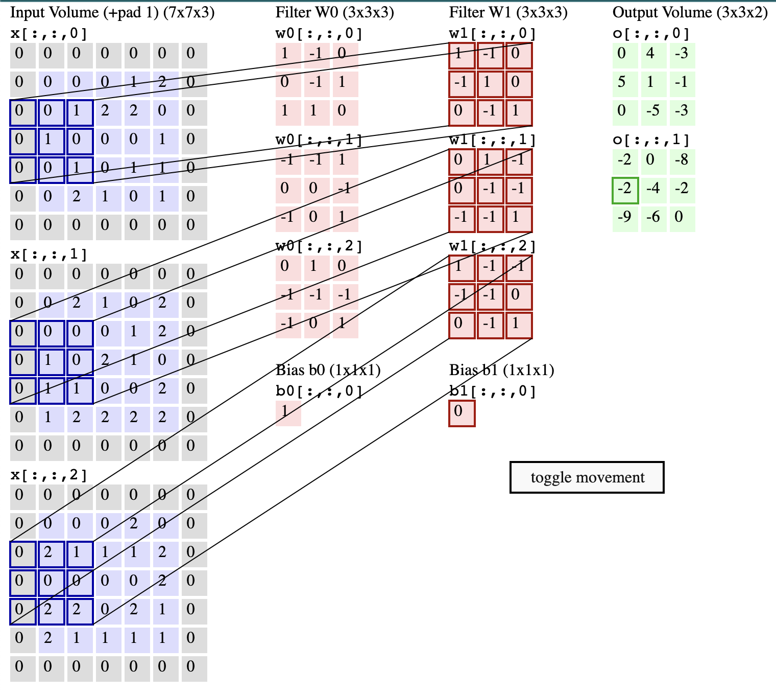
To see this figure animated, clone the class repo and click on the file ./conv-demo/index.html.
Define a Convolutional Neural Network in PyTorch#
We will do the following steps in order:
We already loaded and scaled the MNIST training and test datasets using
torchvisionDefine a Convolutional Neural Network
Define a loss function
Train the network on the training data
Test the network on the test data
# network for MNIST
import torch
from torch import nn

class Net(nn.Module):
    def __init__(self):
        super(Net, self).__init__()
        self.conv1 = nn.Conv2d(1, 32, 3, 1)
        self.conv2 = nn.Conv2d(32, 64, 3, 1)
        self.fc1 = nn.Linear(9216, 128)
        self.fc2 = nn.Linear(128, 10)

    def forward(self, x):
        x = self.conv1(x)
        x = nn.functional.relu(x)
        x = self.conv2(x)
        x = nn.functional.relu(x)
        x = nn.functional.max_pool2d(x, 2)
        x = torch.flatten(x, 1)
        x = self.fc1(x)
        x = nn.functional.relu(x)
        x = self.fc2(x)
        output = nn.functional.log_softmax(x, dim=1)
        return output

net = Net()
Where
CLASS torch.nn.Conv2d(in_channels, out_channels, kernel_size,
                      stride=1, padding_mode='valid', ...)
Layer |
Kernel Size |
Stride |
Input Shape |
Input Channels |
Output Channels |
Output Shape |
|---|---|---|---|---|---|---|
Conv2D/ReLU |
(3x3) |
1 |
28x28 |
1 |
32 |
26x26 |
Conv2D/ReLU |
(3x3) |
1 |
26x26 |
32 |
64 |
24x24 |
Max_pool2d |
(2x2) |
2 |
24x24 |
64 |
64 |
12x12 |
Flatten |
12x12 |
64 |
1 |
9216x1 |
||
FC/ReLU |
9216x1 |
1 |
1 |
128x1 |
||
FC Linear |
128x1 |
1 |
1 |
10x1 |
||
Soft Max |
10x1 |
1 |
1 |
10x1 |

3. Define a Loss function and optimizer#
We’ll use a Classification Cross-Entropy loss and SGD with momentum.
import torch.optim as optim

criterion = nn.CrossEntropyLoss()
optimizer = optim.SGD(net.parameters(), lr=0.001, momentum=0.9)
Cross Entropy Loss#
Popular loss function for multi-class classification that measures the dissimilarity between the predicted class log probability \(\log(p_i)\) and the true class \(y_i\).
See for example here for more information.
Momentum#
Momentum is a technique used in optimizing neural networks that helps accelerate gradients vectors in the right directions, leading to faster convergence. It is inspired by physical laws of motion where the optimizer uses ‘momentum’ to push over hilly terrain and valleys to find the global minimum.
In gradient descent, the weight update rule with momentum is given by:
where:
\(m_t\) is the momentum (which drives the update at iteration \(t\)),
\(\beta \in [0, 1)\), typically 0.9, controls the degree to which the gradient is smoothed over time, and
\(\alpha\) is the learning rate.
See Understanding Deep Learning, Section 6.3 to learn more.
4. Train the network#
print(f"[Epoch #, Iteration #] loss")

# loop over the dataset multiple times
# change this value to 2
for epoch in range(1):

    running_loss = 0.0
    for i, data in enumerate(trainloader, 0):
        # get the inputs; data is a list of [inputs, labels]
        inputs, labels = data

        # zero the parameter gradients
        optimizer.zero_grad()

        # forward + backward + optimize
        outputs = net(inputs)
        loss = criterion(outputs, labels)
        loss.backward()
        optimizer.step()

        # print statistics
        running_loss += loss.item()
        if i % 100 == 99:    # print every 2000 mini-batches
            print(f'[{epoch + 1}, {i + 1:5d}] loss: {running_loss / 2000:.3f}')
            running_loss = 0.0

print('Finished Training')
[Epoch #, Iteration #] loss
[1,   100] loss: 0.108
[1,   200] loss: 0.056
[1,   300] loss: 0.024
[1,   400] loss: 0.019
[1,   500] loss: 0.017
[1,   600] loss: 0.015
[1,   700] loss: 0.014
[1,   800] loss: 0.013
[1,   900] loss: 0.014
[2,   100] loss: 0.011
[2,   200] loss: 0.011
[2,   300] loss: 0.010
[2,   400] loss: 0.009
[2,   500] loss: 0.009
[2,   600] loss: 0.008
[2,   700] loss: 0.008
[2,   800] loss: 0.008
[2,   900] loss: 0.008
Finished Training
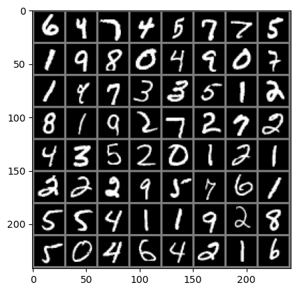
Display some of the images from the test set with the ground truth labels.
dataiter = iter(testloader)
images, labels = next(dataiter)

# print images
imshow(torchvision.utils.make_grid(images))
#print('GroundTruth: ', ' '.join(f'{testset.classes[labels[j]]:5s}' for j in range(4)))
from IPython.display import display, HTML

# Assuming batch_size is 64 and images are displayed in an 8x8 grid
labels_grid = [testset.classes[labels[j]] for j in range(64)]
labels_grid = np.array(labels_grid).reshape(8, 8)

df = pd.DataFrame(labels_grid)

# Generate HTML representation of DataFrame with border
html = df.to_html(border=1)

# Display the DataFrame
display(HTML(html))
| 0 | 1 | 2 | 3 | 4 | 5 | 6 | 7 | |
|---|---|---|---|---|---|---|---|---|
| 0 | 6 - six | 4 - four | 7 - seven | 4 - four | 5 - five | 7 - seven | 7 - seven | 5 - five |
| 1 | 1 - one | 9 - nine | 8 - eight | 0 - zero | 4 - four | 9 - nine | 0 - zero | 7 - seven |
| 2 | 1 - one | 9 - nine | 7 - seven | 3 - three | 3 - three | 5 - five | 1 - one | 2 - two |
| 3 | 8 - eight | 1 - one | 9 - nine | 2 - two | 7 - seven | 2 - two | 7 - seven | 2 - two |
| 4 | 4 - four | 3 - three | 5 - five | 2 - two | 0 - zero | 1 - one | 2 - two | 1 - one |
| 5 | 2 - two | 2 - two | 2 - two | 9 - nine | 5 - five | 7 - seven | 6 - six | 1 - one |
| 6 | 5 - five | 5 - five | 4 - four | 1 - one | 1 - one | 9 - nine | 2 - two | 8 - eight |
| 7 | 5 - five | 0 - zero | 4 - four | 6 - six | 4 - four | 2 - two | 1 - one | 6 - six |
Let’s run inference (forward pass) on the model to get numeric outputs.
outputs = net(images)
Get the index of the element with highest value and print the label associated with that index.
_, predicted = torch.max(outputs, 1)

#print('Predicted: ', ' '.join(f'{testset.classes[predicted[j]]:5s}'
#                              for j in range(4)))
# Assuming batch_size is 64 and images are displayed in an 8x8 grid
labels_grid = [testset.classes[predicted[j]] for j in range(64)]
labels_grid = np.array(labels_grid).reshape(8, 8)

df = pd.DataFrame(labels_grid)

# Generate HTML representation of DataFrame with border
html = df.to_html(border=1)

# Display the DataFrame
display(HTML(html))
| 0 | 1 | 2 | 3 | 4 | 5 | 6 | 7 | |
|---|---|---|---|---|---|---|---|---|
| 0 | 6 - six | 4 - four | 7 - seven | 4 - four | 5 - five | 7 - seven | 7 - seven | 5 - five |
| 1 | 1 - one | 9 - nine | 8 - eight | 0 - zero | 4 - four | 9 - nine | 0 - zero | 7 - seven |
| 2 | 1 - one | 1 - one | 7 - seven | 3 - three | 3 - three | 5 - five | 1 - one | 2 - two |
| 3 | 8 - eight | 1 - one | 9 - nine | 2 - two | 7 - seven | 2 - two | 7 - seven | 2 - two |
| 4 | 4 - four | 3 - three | 5 - five | 2 - two | 0 - zero | 1 - one | 2 - two | 1 - one |
| 5 | 2 - two | 2 - two | 2 - two | 9 - nine | 5 - five | 7 - seven | 6 - six | 1 - one |
| 6 | 5 - five | 5 - five | 4 - four | 1 - one | 1 - one | 9 - nine | 2 - two | 8 - eight |
| 7 | 5 - five | 0 - zero | 4 - four | 6 - six | 4 - four | 2 - two | 1 - one | 6 - six |
Evaluate over the entire test set.
correct = 0
total = 0
# since we're not training, we don't need to calculate the gradients for our outputs
with torch.no_grad():
    for data in testloader:
        images, labels = data
        # calculate outputs by running images through the network
        outputs = net(images)
        # the class with the highest energy is what we choose as prediction
        _, predicted = torch.max(outputs.data, 1)
        total += labels.size(0)
        correct += (predicted == labels).sum().item()

print(f'Accuracy of the network on the 10000 test images: {100 * correct // total} %')
Accuracy of the network on the 10000 test images: 96 %
Evaluate the performance per class.
# prepare to count predictions for each class
correct_pred = {classname: 0 for classname in testset.classes}
total_pred = {classname: 0 for classname in testset.classes}

# again no gradients needed
with torch.no_grad():
    for data in testloader:
        images, labels = data
        outputs = net(images)
        _, predictions = torch.max(outputs, 1)
        # collect the correct predictions for each class
        for label, prediction in zip(labels, predictions):
            if label == prediction:
                correct_pred[testset.classes[label]] += 1
            total_pred[testset.classes[label]] += 1


# print accuracy for each class
for classname, correct_count in correct_pred.items():
    accuracy = 100 * float(correct_count) / total_pred[classname]
    print(f'Accuracy for class: {classname:5s} is {accuracy:.1f} %')
Accuracy for class: 0 - zero is 98.2 %
Accuracy for class: 1 - one is 98.9 %
Accuracy for class: 2 - two is 94.7 %
Accuracy for class: 3 - three is 98.1 %
Accuracy for class: 4 - four is 97.5 %
Accuracy for class: 5 - five is 96.0 %
Accuracy for class: 6 - six is 97.8 %
Accuracy for class: 7 - seven is 96.0 %
Accuracy for class: 8 - eight is 94.3 %
Accuracy for class: 9 - nine is 94.0 %
To Dig Deeper#
Look at common CNN network architectures.
For example in Understanding Deep Learning section 10.5.