NN II – Compute Graph, Backprop and Training#

In this lecture we’ll gradually build out a light weight neural network training framework reminiscent of PyTorch.

We build:

A simple neural network engine we call Value class that wraps numbers and math operators and includes useful attributes and methods for implementing forward pass and back propagation. (~63 lines of code)

We’ll provide (and explain)

A simple compute graph visualization function. (34 lines of code)
A small set of helper functions that easily define a neuron, layer and multi-layer perceptron (MLP). (84 lines of code)

With that we can implement a neural network training loop, and see how similar it is to a PyTorch implementation.

The code is based on Andrej Karpathy’s micrograd.

Neuron and Neural Networks (Recap)#

Now let’s switch gears a bit to define an artificial neuron. For better or worse it is named after and loosely modeled on a biological neuron.

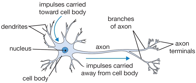
From cs231n

The dendrites carry impulses from other neurons of different distances.
Once the collective firing rate of the impulses exceed a certain threshold, the neuron fires its own pulse through the axon to other neurons

There are companies trying to mimic this impulse (i.e. spiking) based neuron in silicon – so called neuromorphic computing.

See for example Neuromorphic Computing or Spiking Neural Network

Some examples of companies and projects are Intel’s Loihi and startups such as GrAI Matter Labs VIP processor.

Artificial Neuron#

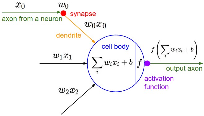
From cs231n

The more common artifical neuron

collects one or more inputs,
each multiplied by a unique weight
sums the weighted inputs
adds a bias
then finally usually applies a nonlinear activation function

Relating Back to Earlier Lectures#

Question

What does

\[\sum_i w_i x_i + b\]

remind you of?

Answer

How about multiple regression in the Linear Regression lecture?

\[y = \beta_0 + \beta_1 u + \beta_2 v\]

We just renamed things: $\beta_0 \gets b$, $\beta_1 \gets w_0$, $\beta_2 \gets w_1$, $u \gets x_0$ and $v \gets x_1$ for $i \in [0,1]$.

So multiple linear regression can be viewed as one linear neuron.

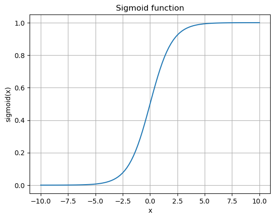
Activation function is typically some nonlinear function that compresses the input in some way. Historically, it’s been the sigmoid and $\tanh()$ functions. See for example Hyperbolic Functions.

import numpy as np
import matplotlib.pyplot as plt

def sigmoid(x):
    return 1 / (1 + np.exp(-x))

x = np.linspace(-10, 10, 100)
y = sigmoid(x)

plt.plot(x, y)
plt.title('Sigmoid function')
plt.xlabel('x')
plt.ylabel('sigmoid(x)')
plt.grid(True)
plt.show()

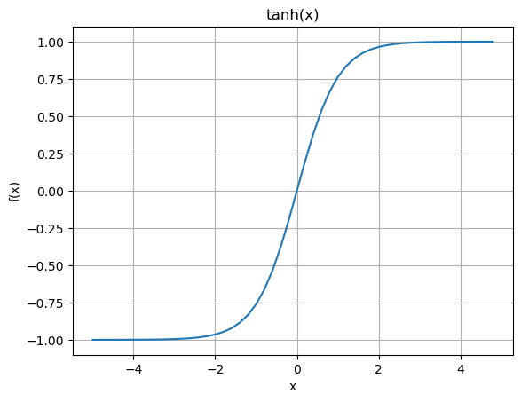
The hyperbolic tangent, $\tanh$, is basically the sigmoid function shifted and scaled to a range of [-1,1].

plt.plot(np.arange(-5,5,0.2), np.tanh(np.arange(-5,5,0.2)))
plt.title('tanh(x)')
plt.xlabel('x')
plt.ylabel('f(x)')
plt.grid()

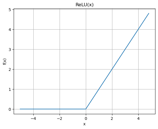
A more common activation function these days and that is more efficient to implement is the Rectified Linear Unit or ReLU.

\[ \textrm{ReLU}(x) = \mathrm{max}(0, x) \]

plt.plot(np.arange(-5,5,0.2), np.maximum(0,np.arange(-5,5,0.2)))
plt.title('ReLU(x)')
plt.xlabel('x')
plt.ylabel('f(x)')
plt.grid()

There are many other variations. See for example PyTorch Non-linear Activations

Relating Back to Another Earlier Lecture#

Question

What does

\[ \mathrm{sigmoid}(\sum_i w_i x_i + b) \hspace{10pt} \textrm{where} \hspace{10pt} \mathrm{sigmoid}(x) = \frac{1}{1 + e^{-x}}\]

remind you of?

Answer

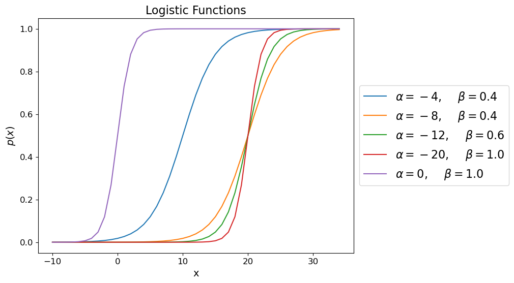
How about the Logistic Regression model?

\[\begin{split} \begin{split} P(y=1\mid x) & = \frac{e^{\alpha+\beta x}}{1+e^{\alpha+\beta x}}\\ & = \frac{e^{\alpha+\beta x}}{1+e^{\alpha+\beta x}} \left( \frac{e^{-(\alpha+\beta x)}}{e^{-(\alpha+\beta x)}} \right) \\ & = \frac{e^{(\alpha+\beta x)-(\alpha+\beta x)}}{e^{-(\alpha+\beta x)}+e^{(\alpha+\beta x)-(\alpha+\beta x)}} \\ & = \frac{e^0}{e^{-(\alpha+\beta x)} + e^0} \\ & = \frac{1}{1 + e^{-(\alpha+\beta x)}} \end{split} \end{split}\]

Which is the Sigmoid with $\alpha = 0$ and $\beta = 1$.

In fact, just like in Logistic Regression, we use the sigmoid function on the last layer of a neural network that is doing binary classification to output the probabilities.

So Logistic Regression is similar to one neuron with a sigmoid activation function.

alphas = [-4, -8,-12,-20, 0]
betas = [0.4,0.4,0.6,1, 1]
x = np.arange(-10,35)
fig = plt.figure(figsize=(8, 6)) 
ax = plt.subplot(111)

for i in range(len(alphas)):
    a = alphas[i]
    b = betas[i]
    y = np.exp(a+b*x)/(1+np.exp(a+b*x))
    ax.plot(x,y,label=r"$\alpha=%d,$    $\beta=%3.1f$" % (a,b))

ax.tick_params(labelsize=12)
ax.set_xlabel('x', fontsize = 14)
ax.set_ylabel('$p(x)$', fontsize = 14)
ax.legend(loc='center left', bbox_to_anchor=(1, 0.5), prop={'size': 16})
ax.set_title('Logistic Functions', fontsize = 16);

Multi-Layer Perceptron (MLP) or Fully Connected Network (FCN)#

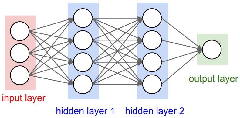
From cs231n

Multiple artificial neurons can be acting on the same inputs, in what we call a layer, and we can have more than one layer until we produce one or more outputs.

The example above shows a network with 3 inputs, two layers of neurons, each with 4 neurons, followed by one layer that produces a single value output.

E.g. a binary classifier.

Computation Graph#

The way we are going to differentiate more complex functions is to first build a “computation graph” to apply our operations on. We’ll see that it breaks down the process into simple steps that easily scale to large networks.

It’s the concept employed by TensorFlow and PyTorch, and in fact we’ll follow PyTorch interface definition.

Building the `Value` Class#

To do that we will build a data wrapper as a class called Value and gradually build in on all the functionality we need to define a Multi-Layer Neural Network (a.k.a. Multi-Layer Perceptron) and train it.

First, the class has only a simple initialization method and a representation method.

# Value version 1
class Value:

    def __init__(self, data):
        self.data = data

    def __repr__(self):
        """Return a string representation of the object for display"""
        return f"Value(data={self.data})"

a = Value(4.0)
a

Value(data=4.0)

If you are not familiar with python classes, there are a few things to note here.

The property self is just a pointer to the object itself.
The __init__ method is called when you initialize a class object
The __repr__ method is how you represent the class object

Implementing Addition#

So the Value object doesn’t do much yet except for taking a value and printing it. We’d also like to do things like addition and other operations with them, but…

a = Value(4.0)
b = Value(-3.0)

try:
    a+b 
except Exception as e:
    print("Uh oh!", e)
else:
    print("It worked!")

Uh oh! unsupported operand type(s) for +: 'Value' and 'Value'

When python tries to add two objects a and b, internally it will call a.__add__(b). So we have to add the __add__() method.

# Value version 2
class Value:

    def __init__(self, data):
        self.data = data

    def __repr__(self):
        """Return a string representation of the object for display"""
        return f"Value(data={self.data})"

    def __add__(self, other):
        other = other if isinstance(other, Value) else Value(other)
        out = Value(self.data + other.data)
        return out

a = Value(4.0)
b = Value(-3.0)

try:
    a+b
except Exception as e:
    print("Uh oh!", e)
else:
    print("It worked!")

It worked!

Which, as mentioned is equivalent to calling the __add__ method on a.

a.__add__(b)

Value(data=1.0)

Implementing More Operations#

Similarly we can support multiplication and implement a ReLU function as well.

import numpy as np

# Value version 3
class Value:

    def __init__(self, data):
        self.data = data

    def __repr__(self):
        """Return a string representation of the object for display"""
        return f"Value(data={self.data})"

    def __add__(self, other): # self + other
        other = other if isinstance(other, Value) else Value(other)
        out = Value(self.data + other.data)
        return out
    
    def __mul__(self, other): # self * other
        other = other if isinstance(other, Value) else Value(other)
        out = Value(self.data * other.data)
        return out
    
    def relu(self):
        out = Value(np.maximum(0, self.data))
        return out

a = Value(4.0)
b = Value(-3.0)
c = Value(8.0)

d = a*b+c
d

Value(data=-4.0)

d.relu()

Value(data=0.0)

By the way, internally, python will call __mul__ on a, then __add__ on the temporary product object.

(a.__mul__(b)).__add__(c)

Value(data=-4.0)

Child Nodes#

In order to calculate the gradients, we will need to capture the computation graphs. To do that, we’ll need to store pointers to the operands of each operation.

To start with, we’ll accept a tuple of child nodes in the initializer and store that as a set in the object.

# Value version 4
class Value:
                        #    vvvvvvvvvvvv
    def __init__(self, data, _children=()):
        self.data = data
        self._prev = set(_children)

    def __repr__(self):
        """Return a string representation of the object for display"""
        return f"Value(data={self.data})"

    def __add__(self, other):
        other = other if isinstance(other, Value) else Value(other)
        out = Value(self.data + other.data, (self, other)) # store tuple of children
        return out                        # ^^^^^^^^^^^^^
    
    def __mul__(self, other):
        other = other if isinstance(other, Value) else Value(other)
        out = Value(self.data * other.data, (self, other)) # store tuple of children
        return out                        # ^^^^^^^^^^^^^
    
    def relu(self):
        out = Value(np.maximum(0, self.data), (self,))
        return out                         #  ^^^^^^^

a = Value(4.0)
b = Value(-3.0)
c = Value(8.0)

d = a*b
e = d + c

We can now see the children of the operands that produced the output value by printing the _prev value. The name _prev might not be intuitive yet, but it will make more sense when we view these operations as a graph.

d._prev

{Value(data=-3.0), Value(data=4.0)}

e._prev

{Value(data=-12.0), Value(data=8.0)}

Child Operations#

Now we’ve recorded pointers to the child nodes. It would be helpful to also record the operator used.

We’ll also add labels for convenience.

# Value version 5
class Value:
                                    #     vvvvvvv  vvvvvvvv
    def __init__(self, data, _children=(), _op='', label=''):
        self.data = data
        self._prev = set(_children)
        self._op = _op # store the operation that created this node
        self.label = label # label for the node

    def __repr__(self):
        """Return a string representation of the object for display"""
        return f"Value(data={self.data})"

    def __add__(self, other):
        other = other if isinstance(other, Value) else Value(other)   
        out = Value(self.data + other.data, (self, other), '+') # store tuple of children
        return out                                      #  ^^^
    
    def __mul__(self, other):
        other = other if isinstance(other, Value) else Value(other)
        out = Value(self.data * other.data, (self, other), '*') # store tuple of children
        return out                                      #  ^^^
    
    def relu(self):                                 #  vvvvvv
        out = Value(np.maximum(0, self.data), (self,), 'ReLU')
        # out = Value(0 if self.data < 0 else self.data, (self,), 'ReLU')

        return out

a = Value(4.0, label='a')
b = Value(-3.0, label='b')
c = Value(8.0, label='c')

d = a*b ; d.label = 'd'
e = d + c ; e.label = 'e'

d._prev, d._op, d.label

({Value(data=-3.0), Value(data=4.0)}, '*', 'd')

e._prev, e._op, e.label

({Value(data=-12.0), Value(data=8.0)}, '+', 'e')

The Compute Graph#

We now have enough information stored about the compute graph to visualize it.

These are two functions to walk the graph and build sets of all nodes and edges (trace) and then draw them as a directed graph (draw_dot).

# draw_dot version 1
from graphviz import Digraph

def trace(root):
  # builds a set of all nodes and set of all edges in a graph
  nodes, edges = set(), set()
  def build(v):
    if v not in nodes:
      nodes.add(v)
      for child in v._prev:
        edges.add((child, v))
        build(child)
  build(root)
  return nodes, edges

def draw_dot(root):
  dot = Digraph(format='svg', graph_attr={'rankdir': 'LR'}) # LR = left to right

  nodes, edges = trace(root)
  for n in nodes:
    uid = str(id(n))
    # for any value in the graph, create a rectangular ('record') node for it
    dot.node(name = uid, label = "{ %s | data %.4f }" % (n.label, n.data), shape='record')
    if n._op:
      # if this value is a result of some operation, create an op node for it
      dot.node(name = uid + n._op, label = n._op)
      # and connect this no de to it
      dot.edge(uid + n._op, uid)

  for n1, n2 in edges:
    # connect n1 to the op node of n2
    dot.edge(str(id(n1)), str(id(n2)) + n2._op)

  return dot

a = Value(4.0, label='a')
b = Value(-3.0, label='b')
c = Value(8.0, label='c')

d = a*b ; d.label = 'd'
e = d + c ; e.label = 'e'

draw_dot(e)

Note that every value object becomes a node in the graph. The operators are also represented as a kind of fake node so they can be visualized too.

nodes, edges = trace(e)
print("Nodes: ", nodes)
print("Edges: ", edges)

Nodes:  {Value(data=-3.0), Value(data=-4.0), Value(data=-12.0), Value(data=8.0), Value(data=4.0)}
Edges:  {(Value(data=4.0), Value(data=-12.0)), (Value(data=-12.0), Value(data=-4.0)), (Value(data=8.0), Value(data=-4.0)), (Value(data=-3.0), Value(data=-12.0))}

Lets add one more operation, or stage in the compute graph.

a = Value(4.0, label='a')
b = Value(-3.0, label='b')
c = Value(8.0, label='c')

d = a*b; d.label = 'd'
e = d + c; e.label = 'e'
f = Value(2.0, label='f')

L = e*f; L.label = 'L'

draw_dot(L)

Recap#

So far we’ve built a Value class and associated data structures to capture a computational graph and calculate the output based on the inputs and operations. We’ll call this the forward pass.

But now, we’re interested in calculating the gradients with respect to some of the parameters with respect to $L$.

So next we’ll update our Value class to capture the partial derivative at each node relative to L.

Calculating Gradients#

Add a gradient member variable, grad, to our class.

# Value version 6
class Value:

    def __init__(self, data, _children=(), _op='', label=''):
        self.data = data
        self.grad = 0.0 # default to 0  <<<<<<<<<<<<<<<<<<<<<<<<<<<<<<<<<<<<<<<<
        self._prev = set(_children)
        self._op = _op # store the operation that created this node
        self.label = label # label for the node

    def __repr__(self):
        """Return a string representation of the object for display"""
        return f"Value(data={self.data})"

    def __add__(self, other):
        other = other if isinstance(other, Value) else Value(other)   
        out = Value(self.data + other.data, (self, other), '+') # store tuple of children
        return out
    
    def __mul__(self, other):
        other = other if isinstance(other, Value) else Value(other)   
        out = Value(self.data * other.data, (self, other), '*') # store tuple of children
        return out
    
    def relu(self):         
        out = Value(np.maximum(0, self.data), (self,), 'ReLU')
        # out = Value(0 if self.data < 0 else self.data, (self,), 'ReLU')

        return out

And update draw_dot() to show grad in the node info.

# draw_dot version 2
from graphviz import Digraph

def trace(root):
  # builds a set of all nodes and set of all edges in a graph
  nodes, edges = set(), set()
  def build(v):
    if v not in nodes:
      nodes.add(v)
      for child in v._prev:
        edges.add((child, v))
        build(child)
  build(root)
  return nodes, edges

def draw_dot(root):
  dot = Digraph(format='svg', graph_attr={'rankdir': 'LR'}) # LR = left to right

  nodes, edges = trace(root)
  for n in nodes:
    uid = str(id(n))
    # for any value in the graph, create a rectangular ('record') node for it
    dot.node(name = uid, label = "{ %s | data %.4f | grad %.4f }" % (n.label, n.data, n.grad), shape='record')
    if n._op:
      # if this value is a result of some operation, create an op node for it
      dot.node(name = uid + n._op, label = n._op)
      # and connect this node to it
      dot.edge(uid + n._op, uid)

  for n1, n2 in edges:
    # connect n1 to the op node of n2
    dot.edge(str(id(n1)), str(id(n2)) + n2._op)

  return dot        

And reinitialize and redraw…

a = Value(4.0, label='a')
b = Value(-3.0, label='b')
c = Value(8.0, label='c')

d = a*b; d.label = 'd'
e = d + c; e.label = 'e'
f = Value(2.0, label='f')

L = e*f; L.label = 'L'

draw_dot(L)

Manual Gradient Calculation#

Before we start implementing backpropagation, it is helpful to manually calculate some gradients to better understand the procedure.

For the node $L$, we trivially calculate $\frac{dL}{dL} = 1$.

From limit ratio perspective,

\[ \frac{\partial L}{\partial L} = \lim_{h \rightarrow 0} \frac{ (L+h) - L }{h} = \frac{h}{h} = 1\]

L.grad = 1.0

If we go backwards a step in the graph, we see that $L=e*f$, so we calculate

\[\frac{\partial{L}}{\partial{e}} = \frac{\partial}{\partial{e}} (e\times f) = f\]

and

\[\frac{\partial{L}}{\partial{f}} = \frac{\partial}{\partial{f}} (e\times f) = e.\]

e.grad = f.data

f.grad = e.data

To summarize, the partial derivative w.r.t. to one operand of a simple product is simply the other operand.

And we can redraw the graph above again.

draw_dot(L)

How do the parameters $e$ and $f$ influence $L$?

# Try uncommenting `e += h` or `f += h` and calling `wiggle()` then `wiggle(1.0)`
# to see the influence of e or f on L
def wiggle(h = 0.0):
    a = Value(4.0, label='a')
    b = Value(-3.0, label='b')
    c = Value(8.0, label='c')

    d = a*b; d.label = 'd'
    e = d + c; e.label = 'e'
    # e += h
    f = Value(2.0, label='f')
    f += h

    L = e*f; L.label = 'L'
    print(L)

wiggle()

Value(data=-8.0)

wiggle(1.0)

Value(data=-12.0)

Propagating Back#

Now we want to calculate

\[\frac{\partial{L}}{\partial{c}}\]

or put another way, we want to know how much $L$ wiggles if we wiggle $c$, or how $c$ influences $L$.

Looking at the graph again we see that $c$ influences $e$ and $e$ influences $L$, so we should be able see the ripple effect of $c$ on $L$.

\[ c \rightarrow e \rightarrow L \]

So $e = c + d$, and so we calculate

\[ \frac{\partial{e}}{\partial{c}} = \frac{\partial{}}{\partial{c}} (d + c) = 1\]

Question#

\[ c \rightarrow e \rightarrow L \]

So now we know $\partial{L}/\partial{e}$ and we also know $\partial{e}/\partial{c}$,

How do we get $\partial{L}/\partial{c}$?

The Chain Rule#

To paraphrase from the Wikipedia page on Chain rule, if a variable $L$ depends on the variable $e$, which itself depends on the variable $c$ (that is, $e$ and $L$ are dependent variables), then $L$ depends on $c$ as well, via the intermediate variable $e$. In this case, the chain rule is expressed as

\[\frac{\partial L}{\partial c} = \frac{\partial L}{\partial e} \cdot \frac{\partial e}{\partial c},\]

and

\[ \left.\frac{\partial L}{\partial c}\right|_{c} = \left.\frac{\partial L}{\partial e}\right|_{e(c)}\cdot \left. \frac{\partial e}{\partial c}\right|_{c} ,\]

for indicating at which points the derivatives have to be evaluated.

Now since we’ve established that

\[ \frac{\partial{e}}{\partial{c}} = 1\]

then

\[\frac{dL}{dc} = \frac{dL}{de} \cdot 1.\]

So in the case of an operand in an addition operation, we just copy the gradient of the parent node.

Or put another way,

in the addition operator, we just route the parent gradient to the child.

d.grad = e.grad
c.grad = e.grad

draw_dot(L)

How does $c$ and $d$ influence $L$?

# Try uncommenting `c += h` or `d += h` and calling `wiggle()` then `wiggle(1.0)`
# to see the influence of c or d on L
def wiggle(h = 0.0):
    a = Value(4.0, label='a')
    b = Value(-3.0, label='b')
    c = Value(8.0, label='c')
    # c += h

    d = a*b; d.label = 'd'
    # d += h

    e = d + c; e.label = 'e'
    f = Value(2.0, label='f')

    L = e*f; L.label = 'L'
    print(L)

wiggle()

Value(data=-8.0)

wiggle(1.0)

Value(data=-8.0)

Propagating Back Again#

Now we want to calculate

\[ \frac{\partial{L}}{\partial{b}} \hspace{10pt} \textrm{and} \hspace{10pt} \frac{\partial{L}}{\partial{a}}\]

But we have

\[ \frac{\partial{L}}{\partial{d}}\]

and we know that

\[ \frac{\partial{d}}{\partial{b}} = \frac{\partial{}}{\partial{b}}(a\cdot b) = a\]

so again from the chain rule

\[\frac{\partial{L}}{\partial{b}} = \frac{\partial{L}}{\partial{d}} \cdot \frac{\partial{d}}{\partial{b}} = \frac{\partial{L}}{\partial{d}} \cdot a\]

b.grad = a.data * d.grad
a.grad = b.data * d.grad
draw_dot(L)

# Try uncommenting `a += h` or `b += h` and calling `wiggle()` then `wiggle(1.0)`
# to see the influence of a or b on L
def wiggle(h = 0.0):
    a = Value(4.0, label='a')
    # a += h
    b = Value(-3.0, label='b')
    b += h
    c = Value(8.0, label='c')

    d = a*b; d.label = 'd'

    e = d + c; e.label = 'e'
    f = Value(2.0, label='f')

    L = e*f; L.label = 'L'
    print(L)

wiggle()

Value(data=-8.0)

wiggle(1.0)

Value(data=0.0)

Recap#

As you saw, we recursively went backwards through the computation graph and applied the local gradients to the gradients calculated so far to get the partial gradients. Put another we propagated this calculations backwards through the graph.

Of course, in practice, we will only need the gradients on the parameters, not the inputs, so we won’t bother calculating them on inputs.

That is the essence of Back Propagation.

A Step in Optimization#

Let’s take a look at the graph again. Assume we want the value of L to decrease. We are free to change the values of the leaf nodes – all the other nodes are derived from children and leaf nodes.

The leaf nodes are $a, b, c$ and $f$.

Again, in practice we would only update the parameter leaf nodes, not the input leaf node, but we’ll ignore that distinction temporarily for this exmaple.

draw_dot(L)

Let’s check the current value of L.

# remind ourselves what L is
print(L.data)

-8.0

As we showed before, we want to nudge each of those leaf nodes by the negative of the gradient, multiplied by a step size, $\eta$.

\[ w_{n+1} = w_n - \eta * \frac{\partial{L}}{\partial{w_n}} \]

where $n$ is the iteration number.

# nudge all the leaf nodes along the negative direction of the gradient
step_size = 0.01    # also called eta above

a.data -= step_size * a.grad
b.data -= step_size * b.grad
c.data -= step_size * c.grad
f.data -= step_size * f.grad

# recompute the forward pass
d = a*b
e = d + c
L = e*f

print(L.data)

-9.230591999999998

A Single Neuron#

Let’s now programmatically define a single neuron with

two inputs
two weights (1 for each input)
a bias
the ReLU activation function

Recall the neuron figure above.

# inputs x0, x1
x1 = Value(2.0, label='x1')
x2 = Value(0.0, label='x2')

# weights w1, w2
w1 = Value(-3.0, label='w1')
w2 = Value(1.0, label='w2')

# bias of the neuron
b = Value(6.8813735870195432, label='b')

x1w1 = x1*w1; x1w1.label = 'x1*w1'
x2w2 = x2*w2; x2w2.label = 'x2*w2'

x1w1x2w2 = x1w1 + x2w2; x1w1x2w2.label = 'x1w1 + x2w2'
n = x1w1x2w2 + b; n.label = 'n'
o = n.relu(); o.label = 'o'

draw_dot(o)

The only new operation we’ve added is the ReLU, so let’s take a quick look at how we differentiate the ReLU.

Like before, for the output node, o:

\[ \frac{\partial o}{\partial o} = 1 \]

o.grad = 1.0

ReLU is technically not differentiable at 0, but practically we implement the derivative as 0 when $ \le 0$ and 1 when $ 1 > 0 $

n.grad = (o.data > 0) * o.grad  # = 0 when o.data <= 0; = o.grad when o.data > 0

Coding Backpropagation#

Now we’ll update our Value class once more to support the backward pass.

There’s a

private _backward() function in each operator that implements the local step of the chain rule, and
a backward() function in the class that topologically sorts the graph and calls the operator _backward() function starting at the end of the graph and going backward.

# version 9
class Value:

    def __init__(self, data, _children=(), _op='', label=''):
        self.data = data
        self.grad = 0.0 # default to 0, no impact on the output
        self._backward = lambda: None  # by default backward doesn't do anything
        self._prev = set(_children)
        self._op = _op
        self.label = label

    def __repr__(self):
        """Return a string representation of the object for display"""
        return f"Value(data={self.data}, grad={self.grad})"

    def __add__(self, other):
        other = other if isinstance(other, Value) else Value(other)
        out = Value(self.data + other.data, (self, other), '+')

        def _backward():
            self.grad += out.grad
            other.grad += out.grad
        out._backward = _backward

        return out

    def __mul__(self, other):
        other = other if isinstance(other, Value) else Value(other)
        out = Value(self.data * other.data, (self, other), '*')

        def _backward():
            self.grad += other.data * out.grad
            other.grad += self.data * out.grad
        out._backward = _backward
        return out

    def relu(self):
        out = Value(np.maximum(0, self.data), (self,), 'ReLU')
        # out = Value(0 if self.data < 0 else self.data, (self,), 'ReLU')

        def _backward():
            self.grad += (out.data > 0) * out.grad
        out._backward = _backward

        return out

    def backward(self):

        # topological order all of the children in the graph
        topo = []
        visited = set()
        def build_topo(v):
            if v not in visited:
                visited.add(v)
                for child in v._prev:
                    build_topo(child)
                topo.append(v)
        build_topo(self)

        # go one variable at a time and apply the chain rule to get its gradient
        self.grad = 1
        for v in reversed(topo):
            v._backward()

We redefined the class so we have to reinitialize the objects and run the operations again.

This constitutes the forward pass.

# inputs x0, x1
x1 = Value(2.0, label='x1')
x2 = Value(0.0, label='x2')

# weights w1, w2
w1 = Value(-3.0, label='w1')
w2 = Value(1.0, label='w2')

# bias of the neuron
#b = Value(6.7, label='b')
b = Value(6.8813735870195432, label='b')

x1w1 = x1*w1; x1w1.label = 'x1*w1'
x2w2 = x2*w2; x2w2.label = 'x2*w2'

x1w1x2w2 = x1w1 + x2w2; x1w1x2w2.label = 'x1w1 + x2w2'
n = x1w1x2w2 + b; n.label = 'n'
o = n.relu(); o.label = 'o'

So we’ve filled the data values for all the nodes, but haven’t calculated the gradients.

draw_dot(o)

Now, all we have to do is call the backward() method of the last node…

o.backward()

And voila! We have all the gradients!

draw_dot(o)

Accumulating the Gradients#

The observant viewer will notice that we are accumulating the gradients.

That is to handle cases like where a Value object is on both sides of the operand like

a = Value(3.0, label='a')
b = a + a ; b.label = 'b'
b.backward()

a

Value(data=3.0, grad=2.0)

If we didn’t have the accumulation, then a.grad = 1 instead.

Or the other case where a node goes to different operations.

a = Value(-2.0, label='a')
b = Value(3.0, label='b')
d = a * b  ; d.label = 'd'
e = a + b   ; e.label = 'e'
  
draw_dot( f) 

You can see analytical verification of the above result in the note in the online book.

The risk now is that if you don’t zero the gradients for the next update iteration, you will have incorrect gradients.

Always remember to zero the gradient in each iteration of the training loop!

Note

We can verify that the gradients are correct analytically.

To find the partial derivative $\frac{\partial f}{\partial a}$, we first need to define $f$ in terms of $a$ and $b$.

Given: $$\begin{aligned} d &= a \times b \\ e &= a + b \\ f &= d \times e \end{aligned}$$

Then $f$ can be expanded as: $$\begin{aligned} f &= (a \times b) \times (a + b) \\ f &= a^2 \times b + a \times b^2 \end{aligned}$$

Next, we find the partial derivative of $f$ with respect to $a$: $$ \frac{\partial f}{\partial a} = 2a \times b + b^2 $$

Finally, we plug in the given values $a = -2.0$ and $b = 3.0$: $$\begin{aligned} \frac{\partial f}{\partial a} &= 2(-2.0) \times 3.0 + 3.0^2 \\ \frac{\partial f}{\partial a} &= -12.0 + 9.0 \\ \frac{\partial f}{\partial a} &= -3.0 \end{aligned}$$

So the partial derivative $\frac{\partial f}{\partial a}$ for the value $a = -2.0$ is $-3.0$.

Enhancements to `Value` Class#

There are still some useful operations that Value doesn’t support, so to be more complete we have the final version of the Value class below.

We added:

__radd__ for when the Value object is the right operand of an add
__rmul__ for when the Value object is the right operand of a product
__pow__ to support the ** operator
plus some others you can see below

# version 9
class Value:

    def __init__(self, data, _children=(), _op='', label=''):
        self.data = data
        self.grad = 0.0 # default to 0, no impact on the output
        self._backward = lambda: None  # by default backward doesn't do anything
        self._prev = set(_children)
        self._op = _op
        self.label = label

    def __add__(self, other):
        other = other if isinstance(other, Value) else Value(other)
        out = Value(self.data + other.data, (self, other), '+')

        def _backward():
            self.grad += out.grad
            other.grad += out.grad
        out._backward = _backward

        return out
    
    def __mul__(self, other):
        other = other if isinstance(other, Value) else Value(other)
        out = Value(self.data * other.data, (self, other), '*')

        def _backward():
            self.grad += other.data * out.grad
            other.grad += self.data * out.grad
        out._backward = _backward
        
        return out

    def __pow__(self, other):
        """Adding support for ** operator, which we'll need for the 
        squared loss function"""
        assert isinstance(other, (int, float)), "only supporting int/float powers for now"
        out = Value(self.data**other, (self,), f'**{other}')

        def _backward():
            self.grad += (other * self.data**(other-1)) * out.grad
        out._backward = _backward

        return out

    def relu(self):
        out = Value(np.maximum(0, self.data), (self,), 'ReLU')
        # out = Value(0 if self.data < 0 else self.data, (self,), 'ReLU')

        def _backward():
            self.grad += (out.data > 0) * out.grad
        out._backward = _backward

        return out

    def __neg__(self): # -self
        return self * -1

    def __radd__(self, other): # other + self
        return self + other

    def __sub__(self, other): # self - other
        return self + (-other)

    def __rsub__(self, other): # other - self
        return other + (-self)

    def __rmul__(self, other): # other * self
        return self * other

    def __truediv__(self, other): # self / other
        return self * other**-1

    def __rtruediv__(self, other): # other / self
        return other * self**-1
    
    def backward(self):

        # topological order all of the children in the graph
        topo = []
        visited = set()
        def build_topo(v):
            if v not in visited:
                visited.add(v)
                for child in v._prev:
                    build_topo(child)
                topo.append(v)
        build_topo(self)

        # go one variable at a time and apply the chain rule to get its gradient
        self.grad = 1
        for v in reversed(topo):
            v._backward()

    def __repr__(self):
        """Return a string representation of the object for display"""
        return f"Value(data={self.data}, grad={self.grad})"

Comparing to PyTorch#

We’re using a class implementation that resembles the PyTorch implementation, and in fact we can compare our implementation with PyTorch.

import torch

x1 = torch.Tensor([2.0]).double()                ; x1.requires_grad = True
x2 = torch.Tensor([0.0]).double()                ; x2.requires_grad = True
w1 = torch.Tensor([-3.0]).double()               ; w1.requires_grad = True
w2 = torch.Tensor([1.0]).double()                ; w2.requires_grad = True
b = torch.Tensor([6.8813735870195432]).double()  ; b.requires_grad = True
n = x1*w1 + x2*w2 + b
o = torch.relu(n)

print(o.data.item())
o.backward()

print('---')
print('x2.grad', x2.grad.item())
print('w2.grad', w2.grad.item())
print('x1.grad', x1.grad.item())
print('w1.grad', w1.grad.item())

0.881373405456543
---
x2.grad 1.0
w2.grad 0.0
x1.grad -3.0
w1.grad 2.0

By default, tensors don’t store gradients and so won’t support backprop, so we explicitly set requires_grad = True.

Neural Network Modules#

Now we’ll define some classes which help us build out a small neural network.

Module – A base class

Neuron – Implement a single linear or nonlinear neuron with nin inputs.

Layer – Implement a layer of network consisting of nout neurons, each taking nin inputs

MLP – A Multi-Layer Perceptron that implements len(nouts) layers of neurons.

Each class can calculate a forward pass and enumerate all its parameters.

import random
# we assume that Value class is already defined

class Module:
    """Define a Neural Network Module base class """

    def zero_grad(self):
        """When we run in a training loop, we'll need to zero out all the gradients
        since they are defined to accumulate in the backwards passes."""
        for p in self.parameters():
            p.grad = 0

    def parameters(self):
        return []

class Neuron(Module):
    """Define a Neuron as a subclass of Module"""

    def __init__(self, nin, nonlin=True):
        """Randomly initialize a set of weights, one for each input, and initialize the bias to zero."""
        self.w = [Value(random.uniform(-1,1)) for _ in range(nin)]
        self.b = Value(0.0)
        self.nonlin = nonlin

    def __call__(self, x):
        """Implement the forward pass of the neuron"""
        act = sum((wi*xi for wi,xi in zip(self.w, x)), self.b)
        return act.relu() if self.nonlin else act

    def parameters(self):
        return self.w + [self.b]

    def __repr__(self):
        return f"{'ReLU' if self.nonlin else 'Linear'}Neuron({len(self.w)})"

class Layer(Module):
    """Define a Layer of Network as a subclass of Module"""

    def __init__(self, nin, nout, **kwargs):
        """Initialize nout Neurons, each with nin inputs"""
        self.neurons = [Neuron(nin, **kwargs) for _ in range(nout)]

    def __call__(self, x):
        """Forward pass each neuron in the layer"""
        out = [n(x) for n in self.neurons]
        return out[0] if len(out) == 1 else out

    def parameters(self):
        return [p for n in self.neurons for p in n.parameters()]

    def __repr__(self):
        return f"Layer of [{', '.join(str(n) for n in self.neurons)}]"

class MLP(Module):
    """Define a Multi-Layer Perceptron"""

    def __init__(self, nin: int, nouts: list):
        """
        Initialize the Multi-Layer Perceptron, by initializing each layer
        then initializing each neuron of each layer.

        Parameters:
            nin: Number of inputs (int)
            nouts: A list of the number of neurons in each layer
        """
        sz = [nin] + nouts
        # self.layers = [Layer(sz[i], sz[i+1]) for i in range(len(nouts))]

        # Create a list of layer objects for this MLP. All but the last layer
        # have ReLU activations. The last layer is linear.
        self.layers = [Layer(sz[i], sz[i+1], nonlin=i!=len(nouts)-1) for i in range(len(nouts))]

    def __call__(self, x):
        """Forward pass through the MLP"""
        for layer in self.layers:
            x = layer(x)
        return x

    def parameters(self):
        """Recursively retrieve the parameters of the MLP"""
        return [p for layer in self.layers for p in layer.parameters()]

    def __repr__(self):
        return f"MLP of [{', '.join(str(layer) for layer in self.layers)}]"

# help(Module)
# Module.__doc__
# help(Neuron)
# help(Layer)
# help(MLP)

Initialize and Evaluate a Neuron#

# 2 inputs
x = [2.0, 3.0]

# initialize neuron with 2 inputs
n = Neuron(2, nonlin=False)

# evaluate our neuron with our 2 inputs
n(x)

Value(data=2.351314740082261, grad=0.0)

LinearNeuron(2)

# list the 2 weights and the bias
n.parameters()

[Value(data=0.5226748811016748, grad=0.0),
 Value(data=0.4353216592929705, grad=0.0),
 Value(data=0.0, grad=0.0)]

Initialize and Evaluate a Layer of Neurons#

# same 2 inputs again
x = [2.0, 3.0]

# Now initialize a layer of 3 neurons, each with 2 inputs
l = Layer(2, 3, nonlin=False)

# Evaluate our layer of neurons with the 2 inputs
l(x)

[Value(data=0.7525061164928648, grad=0.0),
 Value(data=-3.245347683871597, grad=0.0),
 Value(data=0.4281765105075186, grad=0.0)]

Layer of [LinearNeuron(2), LinearNeuron(2), LinearNeuron(2)]

l.parameters()

[Value(data=0.34599955314939446, grad=0.0),
 Value(data=0.020169003398025298, grad=0.0),
 Value(data=0.0, grad=0.0),
 Value(data=-0.15415728894929637, grad=0.0),
 Value(data=-0.9790110353243346, grad=0.0),
 Value(data=0.0, grad=0.0),
 Value(data=-0.06169429508650448, grad=0.0),
 Value(data=0.18385503356017585, grad=0.0),
 Value(data=0.0, grad=0.0)]

Initialize and Evaluate an MLP#

We’ll instantiate an MLP like the picture below.

From cs231n

x = [2.0, 3.0, -1.0]
m = MLP(3, [4, 4, 1])
m(x)

Value(data=-0.018605982977735535, grad=0.0)

MLP of [Layer of [ReLUNeuron(3), ReLUNeuron(3), ReLUNeuron(3), ReLUNeuron(3)], Layer of [ReLUNeuron(4), ReLUNeuron(4), ReLUNeuron(4), ReLUNeuron(4)], Layer of [LinearNeuron(4)]]

# m.parameters()

draw_dot(m(x))

Training Loop#

So after manually iterating, we put it all together in a training loop. We can repeatedly execute the next cell to continue training.

# Define 4 different sets of inputs
xs = [
    [2.0, 3.0, -1.0],
    [3.0, -1.0, 0.5],
    [0.5, 1.0, 1.0],
    [1.0, 1.0, -1.0]
]

# For each input set, we have a desired target value -- binary classification
# ys = [1.0, -1.0, -1.0, 1.0]
ys = [1.0, 0.0, 0.0, 1.0]

# Manually seed the Random Number Generator for Reproducibility
# You can comment the next line out see the variability
np.random.seed(1)

# Initialize an MLP with random weights
m = MLP(3, [4, 4, 1])

losses = []
niters = 100
step_size = 0.01

for k in range(niters):

    # Training Step 1: forward pass
    ypred = [m(x) for x in xs]
    
    # Training Step 2: Calculate the loss
    loss = sum((yout - ygt)**2 for ygt, yout in zip(ys, ypred))
    losses.append(loss.data)

    # Training Step 3: Zero the gradients and run the backward pass
    m.zero_grad()
    loss.backward()

    # Training Step 4: Update parameters
    for p in m.parameters():
        p.data += -step_size * p.grad

    # print(k, loss.data)

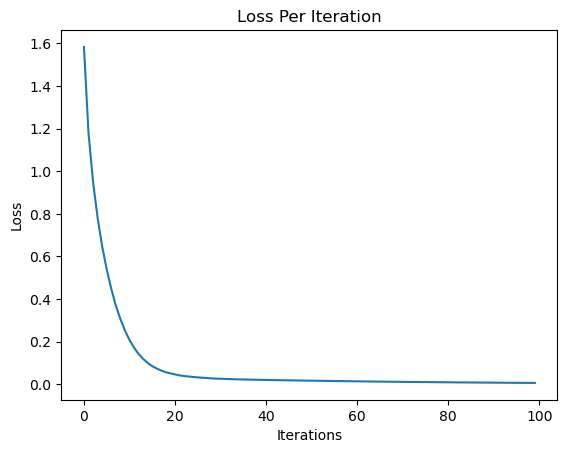
print("Final Loss: ", loss.data)
    
plt.plot(losses)
plt.ylabel("Loss")
plt.xlabel("Iterations")
plt.title("Loss Per Iteration")

Final Loss:  0.005576204735206388

Text(0.5, 1.0, 'Loss Per Iteration')

ypred

[Value(data=1.0366133797239414, grad=0.07322675944788282),
 Value(data=0.00698935172551762, grad=0.01397870345103524),
 Value(data=0.028369351100668988, grad=0.056738702201337976),
 Value(data=0.9418450858397948, grad=-0.11630982832041048)]

Build and Train the Equivalent MLP in PyTorch#

import torch
from torch import nn
from torch.optim import SGD

# Manually seed the Random Number Generator for Reproducibility
# You can comment the next line out see the variability
torch.manual_seed(99)

# Step 1: Define the MLP model
class ptMLP(nn.Module):
    def __init__(self):
        super(ptMLP, self).__init__()
        self.layers = nn.Sequential(
            nn.Linear(3, 4),
            nn.ReLU(),
            nn.Linear(4, 4),
            nn.ReLU(),
            nn.Linear(4, 1)
        )

    def forward(self, x):
        return self.layers(x)

model = ptMLP()
print(model)

# Step 2: Define a loss function and an optimizer
criterion = nn.MSELoss(reduction='sum')
optimizer = SGD(model.parameters(), lr=0.01)

# Step 3: Create a tiny dataset
xs = [
    [2.0, 3.0, -1.0],
    [3.0, -1.0, 0.5],
    [0.5, 1.0, 1.0],
    [1.0, 1.0, -1.0]
]

# we had to transpose ys for torch.tensor
ys_transpose = [[1.0], 
      [0.0], 
      [0.0], 
      [1.0]]

inputs = torch.tensor(xs)
outputs = torch.tensor(ys_transpose)

ptMLP(
  (layers): Sequential(
    (0): Linear(in_features=3, out_features=4, bias=True)
    (1): ReLU()
    (2): Linear(in_features=4, out_features=4, bias=True)
    (3): ReLU()
    (4): Linear(in_features=4, out_features=1, bias=True)
  )
)

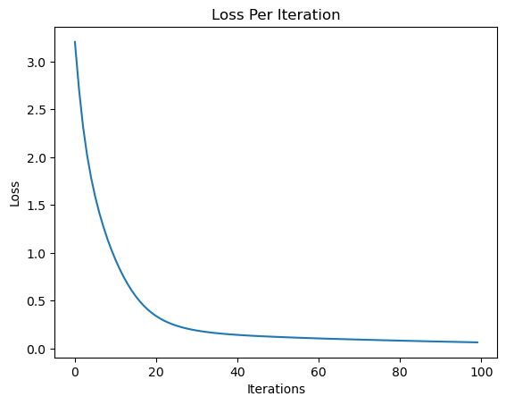
Now run the training loop.

# Step 4: Write the training loop
losses = []
niters = 100

for epoch in range(niters):

    # Training Step 1: Forward pass
    predictions = model(inputs)

    # Training Step 2: Calculate the loss
    loss = criterion(predictions, outputs)

    # Training Step 3: Zero the gradient and run backward pass
    optimizer.zero_grad()
    loss.backward()

    # Training Step 4: Update parameters
    optimizer.step()

    losses.append(loss.item())
    # print(f'Epoch {epoch+1}, Loss: {loss.item()}')

print(f'Final Loss: {loss.item()}')

plt.plot(losses)
plt.ylabel("Loss")
plt.xlabel("Iterations")
plt.title("Loss Per Iteration")

Final Loss: 0.06534020602703094

Text(0.5, 1.0, 'Loss Per Iteration')

predictions

tensor([[1.1306],
        [0.0364],
        [0.0176],
        [0.7840]], grad_fn=<AddmmBackward0>)

To Dig a Little Deeper#

PyTorch Quick Start Tutorial

TensorFlow Playground

Summary#

So today we…

got a glimpse of the wide applications of neural networks
revisited loss functions
developed the notion of gradient descent first by intuition, then in the univariate case, then the multivariate case
defined artificial neurons
implemented a computation graph and visualization
implemented the chain rule as backpropagation on the computation graph
defined Neuron, Layer and MLP modules which completes are homegrown Neural Network Framework
then trained a small MLP on a tiny dataset
finally implemented the same in PyTorch

Tools for Data Science

NN II – Compute Graph, Backprop and Training

Contents

NN II – Compute Graph, Backprop and Training#

Neuron and Neural Networks (Recap)#

Artificial Neuron#

Relating Back to Earlier Lectures#

Relating Back to Another Earlier Lecture#

Multi-Layer Perceptron (MLP) or Fully Connected Network (FCN)#

Computation Graph#

Building the `Value` Class#

Implementing Addition#

Implementing More Operations#

Child Nodes#

Child Operations#

The Compute Graph#

Recap#

Calculating Gradients#

Manual Gradient Calculation#

Propagating Back#

Question#

The Chain Rule#

Propagating Back Again#

Recap#

A Step in Optimization#

A Single Neuron#

Coding Backpropagation#

Accumulating the Gradients#

Enhancements to `Value` Class#

Comparing to PyTorch#

Neural Network Modules#

Initialize and Evaluate a Neuron#

Initialize and Evaluate a Layer of Neurons#

Initialize and Evaluate an MLP#

Training Loop#

Build and Train the Equivalent MLP in PyTorch#

To Dig a Little Deeper#

Summary#

Tools for Data Science

NN II – Compute Graph, Backprop and Training

Contents

NN II – Compute Graph, Backprop and Training#

Neuron and Neural Networks (Recap)#

Artificial Neuron#

Relating Back to Earlier Lectures#

Relating Back to Another Earlier Lecture#

Multi-Layer Perceptron (MLP) or Fully Connected Network (FCN)#

Computation Graph#

Building the Value Class#

Implementing Addition#

Implementing More Operations#

Child Nodes#

Child Operations#

The Compute Graph#

Recap#

Calculating Gradients#

Manual Gradient Calculation#

Propagating Back#

Question#

The Chain Rule#

Propagating Back Again#

Recap#

A Step in Optimization#

A Single Neuron#

Coding Backpropagation#

Accumulating the Gradients#

Enhancements to Value Class#

Comparing to PyTorch#

Neural Network Modules#

Initialize and Evaluate a Neuron#

Initialize and Evaluate a Layer of Neurons#

Initialize and Evaluate an MLP#

Training Loop#

Build and Train the Equivalent MLP in PyTorch#

To Dig a Little Deeper#

Summary#

Building the `Value` Class#

Enhancements to `Value` Class#