Neural Networks I – Gradient Descent
Contents
Neural Networks I – Gradient Descent#
The “Unreasonable” Effectiveness of Deep Neural Networks#
Deep Neural Networks have been effective in many applications.


Understanding Deep Learning, Simon J.D. Prince, MIT Press, 2023
Emergent Behavior in Pre-Trained Large Language Models#
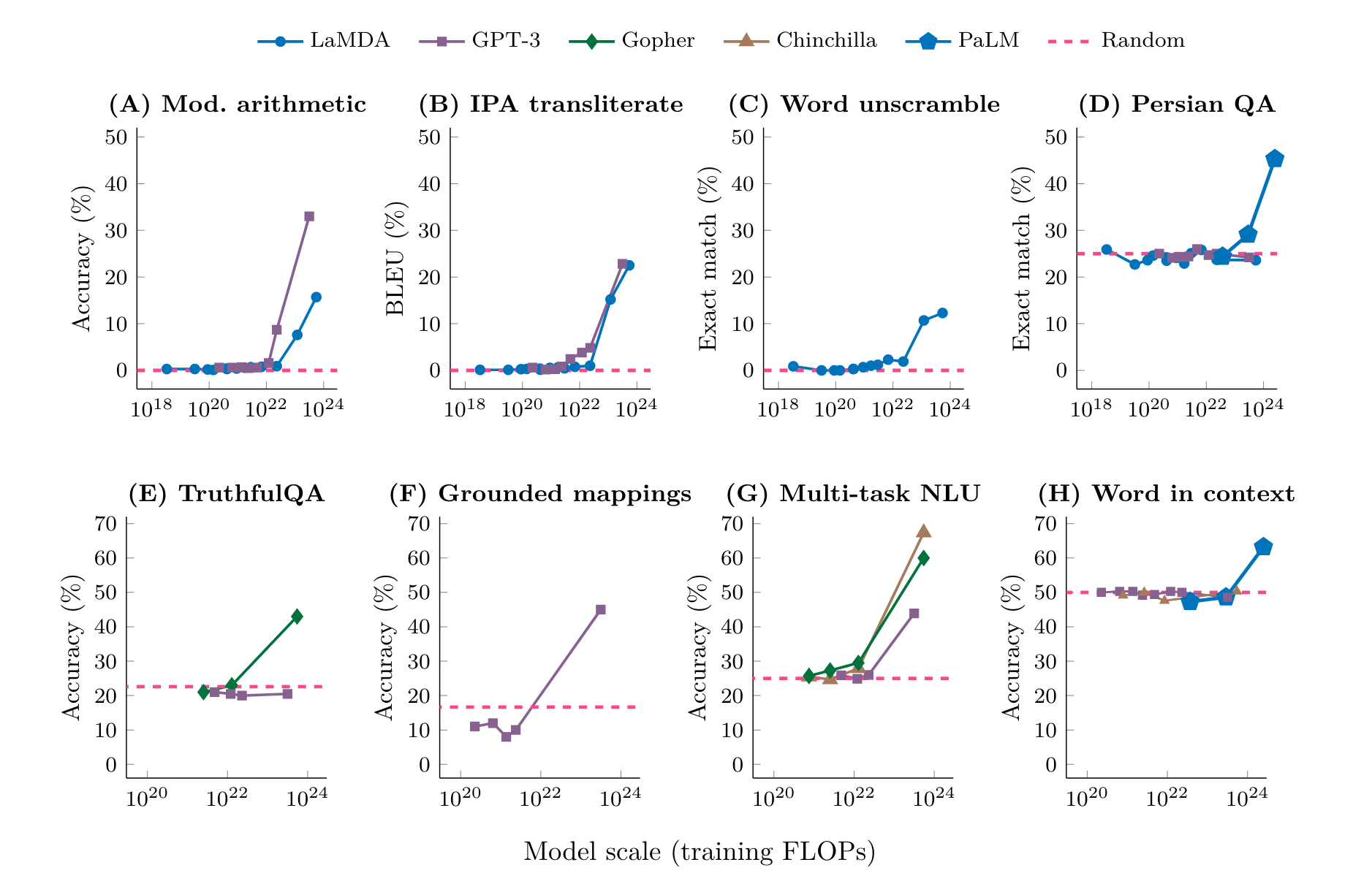
Emergent Abilities of Large Language Models. J. Wei et al., Oct. 26, 2022.
Theory Sometimes Follows Invention#
Invention |
Theory |
|---|---|
Telescope (1608) |
Optics (1650-1700) |
Steam Engine (1695-1715) |
Thermodynamics (1824…) |
Electromagnetism (1820) |
Electrodynamics (1821) |
Sailboat (??) |
Aerodynamics (1757), Hydrodynamics (1738) |
Airplane (1885-1905) |
Wing Theory (1907-1918) |
Computer (1941-1945) |
Computer Science (1950-1960) |
Teletype (1906) |
Information Theory (1948) |
But then when theory is developed it can more quickly improve invention
The same can be said for Neural Networks. The theory to make them work is well understood. The theory of why they work is still developing.
We’ll balance theory and application
The Power and Limits of Deep Learning, Yann LeCun, March 2019.
Underlying all these techniques is the idea of applying optimization techniques to minimize some kind of “loss” function.
Loss Functions for Model Fitting#
Most of the machine learning we have studied this semester is based on the idea that we have a model that is parameterized, and our goal is to find good settings for the parameters.
We have seen example after example of this problem.
In \(k\)-means, our goal was to find \(k\) cluster centroids, so that the \(k\)-means objective was minimized.
In linear regression, our goal was to find a parameter vector \(\beta\) so that sum of squared error \(\Vert \mathbf{y} - \hat{\mathbf{y}}\Vert_2\) was minimized.
In the support vector machine, our goal was to find a parameter vector \(\theta\) so that classification error was minimized.
And similarly we’ll want to find good parameter settings in neural networks.
It’s time now to talk about how, in general, one can find “good settings” for the parameters in problems like these.
What allows us to unify our approach to many such problems is the following:
First, we start by defining an error function, generally called a loss function, to describe how well our method is doing.
And second, we choose loss functions that are differentiable with respect to the parameters.
These two requirements mean that we can think of the parameter tuning problem using surfaces like these:

Imagine that the \(x\) and \(y\) axes in these pictures represent parameter settings. That is, we have two parameters to set, corresponding to the values of \(x\) and \(y\).
For each \((x, y)\) setting, the \(z\)-axis shows the value of the loss function.
What we want to do is find the minimum of a surface, corresponding to the parameter settings that minimize loss.
Notice the difference between the two kinds of surfaces.
The surface on the left corresponds to a strictly convex loss function. If we find a local minimum of this function, it is a global minimum.
The surface on the right corresponds to a non-convex loss function. There are local minima that are not globally minimal.
Both kinds of loss functions arise in machine learning.
For example, convex loss functions arise in
Linear regression
Logistic regression
While non-convex loss functions arise in
\(k\)-means
Gaussian Mixture Modeling
and of course neural networks
Gradient Descent Intuitively#
The intuition of gradient descent is the following.
Imagine you are lost in the mountains, and it is foggy out. You want to find a valley. But since it is foggy, you can only see the local area around you.

The natural thing to do is:
Look around you 360 degrees.
Observe in which direction the ground is sloping downward most steeply.
Take a few steps in that direction.
Repeat the process
… until the ground seems to be level.
The key to this intuitive idea is formalizing the idea of “direction of steepest descent.”
This is where the differentiability of the loss function comes into play.
As long as the loss function is locally differentiable, we can define the direction of steepest descent (really, ascent).
That direction is called the gradient.
Derivatives on Single Variable Functions#
We’ll build up to concept of gradient by starting with derivatives on single variable functions.
Let’s start with a simple quadratic function.
Which we can write in python as well.
def f(x):
return 3*x**2 - 4*x + 5
And we can plot it.
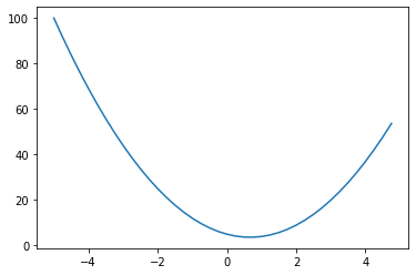
Let’s assume for a minute that this is our loss function that we are minimizing.
Question
What do we know about where the minimum is in terms of the slope of the curve?
Answer
It is necessary but not sufficient that the slope be zero.
Question
How do we calculate the slope?
We take the derivative, denoted
or $\( f'(x) \hspace{10pt} \textrm{Lagrange's notation} \)$
You may see both notations. The nice thing about Leibniz’ notation is that it is easy to express partial derivatives when we get to multivariate differentiation, which we’ll get to shortly.
We can take the derivate of the \(f(x)\)
By definition of the derivative, the function \(f(x)\) is differentiable at \(x\) if
exists at \(x\). And in fact, that limit approaches the value of the derivative in the limit.
We use the rules of derivatives. See for example the derivative rules for basic functions, e.g.
so
# define the derivate of f as df
def df(x):
return 6*x - 4
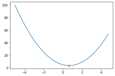
We can solve for where \(\frac{d}{dx} f(x) = 0\)
# Evaluate df and f for x where df = 0
x_zero = 2/3
# Evaluate df
df(x_zero)
0.0
# And f at that value is
f(x_zero)
3.666666666666667
Which we can add to the plot of \(f(x)\) to see if it indeed is at the minimum.
Now as Wikipedia states,
The derivative of a function of a single variable at a chosen input value, when it exists, is the slope of the tangent line to the graph of the function at that point.
Slope of a Function#
We can explore the tangent at different x-values.
Slope Shows Influence of \(x\) on \(f\)#
Important Note:
if the slope is negative, then by increasing \(x\), we will decrease \(f(x)\).
And if the slope is positive, then decreasing \(x\) will decrease \(f(x)\).
Interpretation of Slope#
Let’s illustrate with this function \(f(x)\) a useful way to interpret the slope.
In the graph above, with \(x=-2\), we see the slope, call it \(m\), is -16. What that means is that when we change the value of \(x\), the impact on the ouptut will roughly be amplified by \(m\), or -16 when \(x=2\).
Put another way, the slope (equivalently the derivative) of a function \(f(x)\) at an input \(x\) indicates how sensitive the output is to changes in the input.
This will be key to understanding how we have to tweak the weights of our model to minimize our loss function.
Gradient Descent on a Linear Regression Model#
Now, in 2 or higher dimensions we can there many directions that will descend, but we want to pick the direction of steepest descent. We’ll formalize that idea.
As long as the loss function is locally differentiable, we can define the direction of steepest descent.
That direction is given by the negative of the gradient.
The gradient is a generalization of the slope of a line.
Let’s say we have a loss function \(\mathcal{L}(\mathbf{w})\).
The components of \(\mathbf{w}\in\mathbb{R}^n\) are the parameters we want to optimize.
Just a reminder that \( \mathbf{w} \in \mathbb{R}^n \) denotes an n-dimensional vector.
For linear regression, the loss function could be squared loss:
where \(\hat{\mathbf{y}}\) is our estimate, ie, \(\hat{\mathbf{y}} = X\mathbf{w}\) so that
To find the gradient, we take the partial derivative of our loss function with respect to each parameter:
and collect all the partial derivatives into a vector of the same shape as \(\mathbf{w}\):
When you see the notation \(\nabla_\mathbf{w}\mathcal{L},\) think of it as the derivate with respect to the vector \(\mathbf{w}\).
The nabla symbol, \(\nabla\), denotes the vector differentiator operator called del.
It turns out that if we are going to take a small step of unit length, then the gradient is the direction that maximizes the change in the loss function.

As you can see from the above figure, in general the gradient varies depending on where you are in the parameter space.
So we write:
Each time we seek to improve our parameter estimates \(\mathbf{w}\), we will take a step in the negative direction of the gradient.
… “negative direction” because the gradient specifies the direction of maximum increase – and we want to decrease the loss function.
How big a step should we take?
For step size, will use a scalar value, here denoted by the greek letter “eta”, \(\eta\), which we call the learning rate.
The learning rate is a hyperparameter that needs to be tuned for a given problem, or even can be modified adaptively as the algorithm progresses as we will see later.
Now we can write the gradient descent algorithm formally:
Start with an initial parameter estimate \(\mathbf{w}^0\).
Update: \(\mathbf{w}^{n+1} = \mathbf{w}^n - \eta \nabla_\mathbf{w}\mathcal{L}(\mathbf{w}^n)\)
If not converged, go to step 2.
How do we know if we are “converged”?
Typically we stop
after a certain number of iterations, or
the loss has not improved by a fixed amount – early stopping
Example: Linear Regression#
Let’s say we have this dataset.
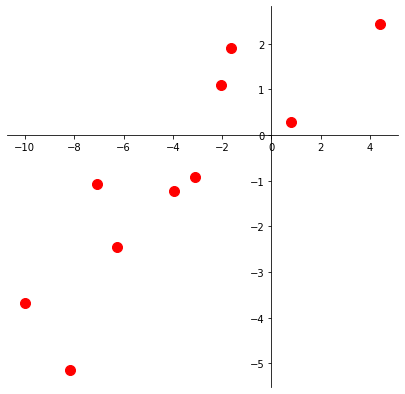
Let’s fit a least-squares line to this data.
The loss function for this problem is the least-squares error:
Of course, we know how to solve this problem using the normal equations, but let’s do it using gradient descent instead.
Here is the line we’d like to find:
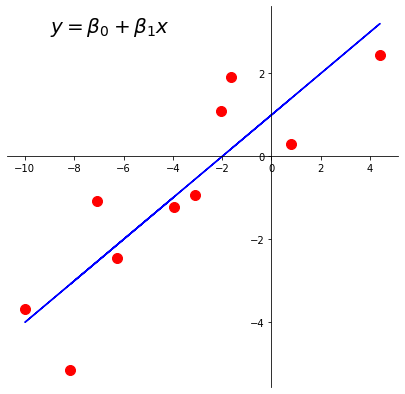
There are \(n = 10\) data points, whose \(x\) and \(y\) values are stored in xlin and y.
First, let’s create our \(X\) (design) matrix, and include a column of ones to model the intercept:
X = np.column_stack([np.ones((n, 1)), xlin])
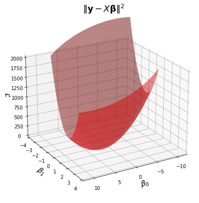
Now, let’s visualize the loss function \(\mathcal{L}(\mathbf{\beta}) = \Vert \mathbf{y}-X\mathbf{\beta}\Vert^2.\)
We won’t take you through computing the gradient for this problem (you can find it in the online text).
We’ll will just tell you that the gradient for a least squares problem is:
Note
For those interested in a little more insight into what these plots are showing, here is the derivation.
We start from the rule that \(\Vert \mathbf{v}\Vert = \sqrt{\mathbf{v}^T\mathbf{v}}\).
Applying this rule to our loss function:
The first term, \(\beta^T X^T X \beta\), is a quadratic form, and it is what makes this surface curved. As long as \(X\) has independent columns, \(X^TX\) is positive definite, so the overall shape is a paraboloid opening upward, and the surface has a unique minimum point.
To find the gradient, we can use standard calculus rules for derivates involving vectors. The rules are not complicated, but the bottom line is that in this case, you can almost use the same rules you would if \(\beta\) were a scalar:
And by the way – since we’ve computed the derivative as a function of \(\beta\), instead of using gradient descent, we could simply solve for the point where the gradient is zero. This is the optimal point which we know must exist:
Which of course, are the normal equations for this linear system.
So here is our code for gradient descent:
def loss(X, y, beta):
return np.linalg.norm(y - X @ beta) ** 2
def gradient(X, y, beta):
return X.T @ X @ beta - X.T @ y
def gradient_descent(X, y, beta_hat, eta, nsteps = 1000):
losses = [loss(X, y, beta_hat)]
betas = [beta_hat]
#
for step in range(nsteps):
#
# the gradient step
new_beta_hat = beta_hat - eta * gradient(X, y, beta_hat)
beta_hat = new_beta_hat
#
# accumulate statistics
losses.append(loss(X, y, new_beta_hat))
betas.append(new_beta_hat)
return np.array(betas), np.array(losses)
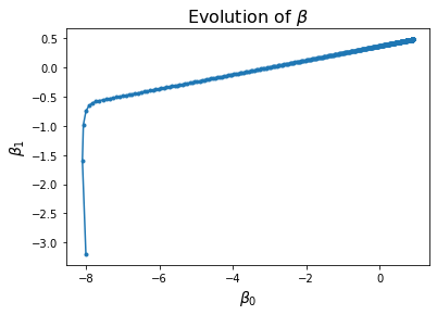
We’ll start at an arbitrary point, say, \((-8, -3.2)\).
That is, \(\beta_0 = -8\), and \(\beta_1 = -3.2\).
beta_start = np.array([-8, -3.2])
eta = 0.002
betas, losses = gradient_descent(X, y, beta_start, eta)
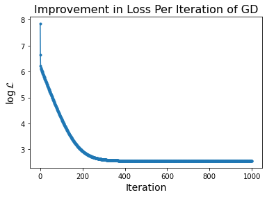
What happens to our loss function per GD iteration?
And how do the parameter values \(\beta\) evolve?
Notice that the improvement in loss decreases over time. Initially the gradient is steep and loss improves fast, while later on the gradient is shallow and loss doesn’t improve much per step.
Now remember that in reality we are like the person who is trying to find their way down the mountain, in the fog.
In general we cannot “see” the entire loss function surface.
Nonetheless, since we know what the loss surface looks like in this case, we can visualize the algorithm “moving” on that surface.
This visualization combines the last two plots into a single view.