Symmetric Matrices
Many parts of this page are based on Linear Algebra and its Applications, by David C. Lay
Today we’ll study a very important class of matrices: symmetric matrices.
We’ll see that symmetric matrices have properties that relate to both eigendecomposition, and orthogonality.
Furthermore, symmetric matrices open up a broad class of problems we haven’t yet touched on: constrained optimization.
As a result, symmetric matrices arise very often in applications.
Definition. A symmetric matrix is a matrix \(A\) such that \(A^T = A\).
Clearly, such a matrix is square.
Furthermore, the entries that are not on the diagonal come in pairs, on opposite sides of the diagonal.
Example. Here are three symmetric matrices:
\[\begin{bmatrix}1&0\\0&-3\end{bmatrix},\;\;\;\;\begin{bmatrix}0&-1&0\\-1&5&8\\0&8&-7\end{bmatrix},\;\;\;\;\begin{bmatrix}a&b&c\\b&d&e\\c&e&f\end{bmatrix}\]
Here are three nonsymmetric matrices:
\[\begin{bmatrix}1&-3\\3&0\end{bmatrix},\;\;\;\;\begin{bmatrix}0&-4&0\\-6&1&-4\\0&-6&1\end{bmatrix},\;\;\;\;\begin{bmatrix}5&4&3&2\\4&3&2&1\\3&2&1&0\end{bmatrix}\]
Orthogonal Diagonalization
At first glance, a symmetric matrix may not seem that special!
But in fact symmetric matrices have a number of very nice properties.
First, we’ll look at a remarkable fact:
the eigenvectors of a symmetric matrix are orthogonal
Example. Let’s diagonalize the following symmetric matrix:
\[A = \begin{bmatrix}6&-2&-1\\-2&6&-1\\-1&-1&5\end{bmatrix}\]
Solution.
The characteristic equation of \(A\) is
\[0 = -\lambda^3 + 17\lambda^2 -90\lambda + 144 \]
\[ = -(\lambda-8)(\lambda-6)(\lambda-3)\]
So the eigenvalues are 8, 6, and 3.
We construct a basis for each eigenspace:
(using our standard method of finding the nullspace of \(A-\lambda I\))
\[\lambda_1 = 8: \mathbf{v}_1 = \begin{bmatrix}-1\\1\\0\end{bmatrix};\;\;\;\;\lambda_2=6: \mathbf{v}_2 = \begin{bmatrix}-1\\-1\\2\end{bmatrix};\;\;\;\;\;\lambda_3=3: \mathbf{v}_3=\begin{bmatrix}1\\1\\1\end{bmatrix}\]
These three vectors form a basis for \(\mathbb{R}^3.\)
But here is the remarkable thing: these three vectors form an orthogonal set.
That is, any two of these eigenvectors are orthogonal.
For example,
\[\mathbf{v}_1^T\mathbf{v}_2 = (-1)(-1) + (1)(-1) + (0)(2) = 0\]
As a result, \(\{\mathbf{v}_1, \mathbf{v}_2, \mathbf{v}_3\}\) form an orthogonal basis for \(\mathbb{R}^3.\)
Let’s normalize these vectors so they each have length 1:
\[\mathbf{u}_1 = \begin{bmatrix}-1/\sqrt{2}\\1/\sqrt{2}\\0\end{bmatrix};\;\;\;\;\mathbf{u}_2 = \begin{bmatrix}-1/\sqrt{6}\\-1/\sqrt{6}\\2/\sqrt{6}\end{bmatrix};\;\;\;\;\; \mathbf{u}_3=\begin{bmatrix}1/\sqrt{3}\\1/\sqrt{3}\\1/\sqrt{3}\end{bmatrix}\]
The orthogonality of the eigenvectors of a symmetric matrix is quite important.
To see this, let’s write the diagonalization of \(A\) in terms of these eigenvectors and eigenvalues:
\[P = \begin{bmatrix}-1/\sqrt{2}&-1/\sqrt{6}&1/\sqrt{3}\\1/\sqrt{2}&-1/\sqrt{6}&1/\sqrt{3}\\0&2/\sqrt{6}&1/\sqrt{3}\end{bmatrix},\;\;\;\;D = \begin{bmatrix}8&0&0\\0&6&0\\0&0&3\end{bmatrix}.\]
Then, \(A = PDP^{-1},\) as usual.
But, here is the interesting thing:
\(P\) is square and has orthonormal columns.
So \(P\) is an orthogonal matrix.
So, that means that \(P^{-1} = P^T.\)
So, \(A = PDP^T.\)
This is a remarkably simple factorization of \(A\).
The Spectral Theorem
It’s not a coincidence that the \(P\) matrix was orthogonal.
In fact we always get orthogonal eigenvectors when we diagonalize a symmetric matrix.
Theorem. If \(A\) is symmetric, then any two eigenvectors of \(A\) from different eigenspaces are orthogonal.
Proof.
Let \(\mathbf{v}_1\) and \(\mathbf{v}_2\) be eigenvectors that correspond to distinct eigenvalues, say, \(\lambda_1\) and \(\lambda_2.\)
To show that \(\mathbf{v}_1^T\mathbf{v}_2 = 0,\) compute
\[\lambda_1\mathbf{v}_1^T\mathbf{v}_2 = (\lambda_1\mathbf{v}_1)^T\mathbf{v}_2\]
\[=(A\mathbf{v}_1)^T\mathbf{v}_2\]
\[=(\mathbf{v}_1^TA^T)\mathbf{v}_2\]
\[=\mathbf{v}_1^T(A\mathbf{v}_2)\]
\[=\mathbf{v}_1^T(\lambda_2\mathbf{v}_2)\]
\[=\lambda_2\mathbf{v}_1^T\mathbf{v}_2\]
So we conclude that \(\lambda_1(\mathbf{v}_1^T\mathbf{v}_2) = \lambda_2(\mathbf{v}_1^T\mathbf{v}_2).\)
But \(\lambda_1 \neq \lambda_2,\) so this can only happen if \(\mathbf{v}_1^T\mathbf{v}_2 = 0.\)
So \(\mathbf{v}_1\) is orthogonal to \(\mathbf{v}_2.\)
The same argument applies to any other pair of eigenvectors with distinct eigenvalues.
So any two eigenvectors of \(A\) from different eigenspaces are orthogonal.
We can now introduce a special kind of diagonalizability:
An \(n\times n\) matrix is said to be orthogonally diagonalizable if there are an orthogonal matrix \(P\) (with \(P^{-1} = P^T\)) and a diagonal matrix \(D\) such that
\[A = PDP^T = PDP^{-1}\]
Such a diagonalization requires \(n\) linearly independent and orthonormal eigenvectors.
When is it possible for a matrix’s eigenvectors to form an orthogonal set?
Well, if \(A\) is orthogonally diagonalizable, then
\[A^T = (PDP^T)^T = (P^T)^TD^TP^T = PDP^T = A\]
So \(A\) is symmetric!
That is, whenever \(A\) is orthogonally diagonalizable, it is symmetric.
It turns out the converse is true (though we won’t prove it): every symmetric matrix is orthogonally diagonalizable.
Hence we obtain the following important theorem:
Theorem. An \(n\times n\) matrix is orthogonally diagonalizable if and only if it is a symmetric matrix.
Remember that when we studied diagonalization, we found that it was a difficult process to determine if an arbitrary matrix was diagonalizable.
But here, we have a very nice rule: every symmetric matrix is (orthogonally) diagonalizable.
Quadratic Forms
An important reason to study symmetric matrices has to do with quadratic expressions.
Up until now, we have mainly focused on linear equations – equations in which the \(x_i\) terms occur only to the first power.
Actually, though, we have looked at some quadratic expressions when we considered least-squares problems.
For example, we looked at expressions such as \(\Vert x\Vert^2\) which is \(\sum x_i^2.\)
We’ll now look at quadratic expressions generally. We’ll see that there is a natural and useful connection to symmetric matrices.
Definition. A quadratic form is a function of variables, eg, \(x_1, x_2, \dots, x_n,\) in which every term has degree two.
Examples:
\(4x_1^2 + 2x_1x_2 + 3x_2^2\) is a quadratic form.
\(4x_1^2 + 2x_1\) is not a quadratic form.
Quadratic forms arise in many settings, including signal processing, physics, economics, and statistics.
In computer science, quadratic forms arise in optimization and graph theory, among other areas.
Essentially, what an expression like \(x^2\) is to a scalar, a quadratic form is to a vector.
Fact. Every quadratic form can be expressed as \(\mathbf{x}^TA\mathbf{x}\), where \(A\) is a symmetric matrix.
There is a simple way to go from a quadratic form to a symmetric matrix, and vice versa.
To see this, let’s look at some examples.
Example. Let \(\mathbf{x} = \begin{bmatrix}x_1\\x_2\end{bmatrix}.\) Compute \(\mathbf{x}^TA\mathbf{x}\) for the matrix \(A = \begin{bmatrix}4&0\\0&3\end{bmatrix}.\)
Solution.
\[\mathbf{x}^TA\mathbf{x} = \begin{bmatrix}x_1&x_2\end{bmatrix}\begin{bmatrix}4&0\\0&3\end{bmatrix}\begin{bmatrix}x_1\\x_2\end{bmatrix}\]
\[= \begin{bmatrix}x_1&x_2\end{bmatrix}\begin{bmatrix}4x_1\\3x_2\end{bmatrix}\]
\[= 4x_1^2 + 3x_2^2.\]
Example. Compute \(\mathbf{x}^TA\mathbf{x}\) for the matrix \(A = \begin{bmatrix}3&-2\\-2&7\end{bmatrix}.\)
Solution.
\[\mathbf{x}^TA\mathbf{x} = \begin{bmatrix}x_1&x_2\end{bmatrix}\begin{bmatrix}3&-2\\-2&7\end{bmatrix}\begin{bmatrix}x_1\\x_2\end{bmatrix}\]
\[=x_1(3x_1 - 2x_2) + x_2(-2x_1 + 7x_2)\]
\[=3x_1^2-2x_1x_2-2x_2x_1+7x_2^2\]
\[=3x_1^2-4x_1x_2+7x_2^2\]
Notice the simple structure:
\[a_{11} \text{ is multiplied by } x_1 x_1\]
\[a_{12} \text{ is multiplied by } x_1 x_2\]
\[a_{21} \text{ is multiplied by } x_2 x_1\]
\[a_{22} \text{ is multiplied by } x_2 x_2\]
We can write this concisely:
\[ \mathbf{x}^TA\mathbf{x} = \sum_{ij} a_{ij}x_i x_j \]
Example. For \(\mathbf{x}\) in \(\mathbb{R}^3\), let
\[Q(\mathbf{x}) = 5x_1^2 + 3x_2^2 + 2x_3^2 - x_1x_2 + 8x_2x_3.\]
Write this quadratic form \(Q(\mathbf{x})\) as \(\mathbf{x}^TA\mathbf{x}\).
Solution.
The coefficients of \(x_1^2, x_2^2, x_3^2\) go on the diagonal of \(A\).
Based on the previous example, we can see that the coefficient of each cross term \(x_ix_j\) is the sum of two values in symmetric positions on opposite sides of the diagonal of \(A\).
So to make \(A\) symmetric, the coefficient of \(x_ix_j\) for \(i\neq j\) must be split evenly between the \((i,j)\)- and \((j,i)\)-entries of \(A\).
You can check that for
\[Q(\mathbf{x}) = 5x_1^2 + 3x_2^2 + 2x_3^2 - x_1x_2 + 8x_2x_3\]
that
\[Q(\mathbf{x}) = \mathbf{x}^TA\mathbf{x} = \begin{bmatrix}x_1&x_2&x_3\end{bmatrix}\begin{bmatrix}5&-1/2&0\\-1/2&3&4\\0&4&2\end{bmatrix}\begin{bmatrix}x_1\\x_2\\x_3\end{bmatrix}\]
Classifying Quadratic Forms
Notice that \(\mathbf{x}^TA\mathbf{x}\) is a scalar.
In other words, when \(A\) is an \(n\times n\) matrix, the quadratic form \(Q(\mathbf{x}) = \mathbf{x}^TA\mathbf{x}\) is a real-valued function with domain \(\mathbb{R}^n\).
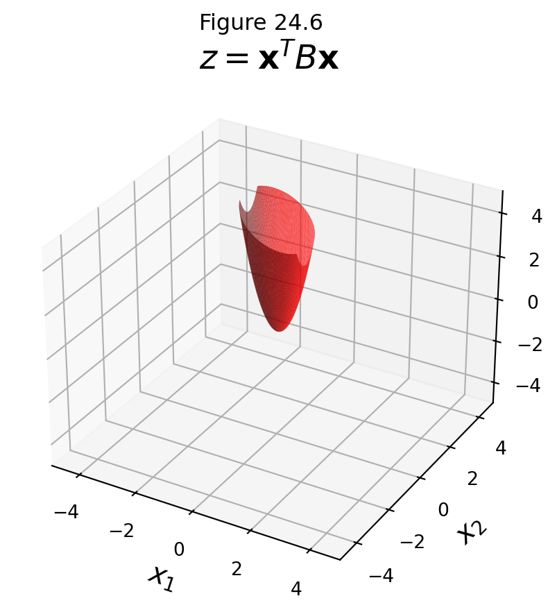
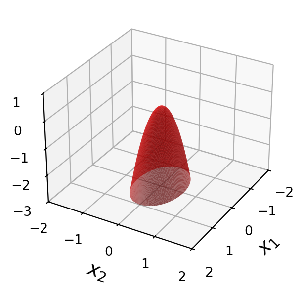
Here are four quadratic forms with domain \(\mathbb{R}^2\).
Notice that except at \(\mathbf{x}=\mathbf{0},\) the values of \(Q(\mathbf{x})\) are all positive in the first case, and all negative in the last case.
The differences between these surfaces is important for problems such as optimization.
In an optimization problem, one seeks the minimum or maximum value of a function (perhaps over a subset of its domain).
Definition. A quadratic form \(Q\) is:
1. positive definite if \(Q(\mathbf{x}) > 0\) for all \(\mathbf{x} \neq 0.\)
2. positive semidefinite if \(Q(\mathbf{x}) \geq 0\) for all \(\mathbf{x} \neq 0.\)
3. indefinite if \(Q(\mathbf{x})\) assumes both positive and negative values.
4. negative semidefinite if \(Q(\mathbf{x}) \leq 0\) for all \(\mathbf{x} \neq 0.\)
5. negative definite if \(Q(\mathbf{x}) < 0\) for all \(\mathbf{x} \neq 0.\)
Classifying Quadratic Forms
Knowing which kind of quadratic form one is dealing with is important for optimization.
Consider these two quadratic forms:
\[ P(\mathbf{x}) = \mathbf{x}^TA\mathbf{x}, \text{ where } A = \begin{bmatrix}3&2\\2&1\end{bmatrix} \]
\[ Q(\mathbf{x}) = \mathbf{x}^TB\mathbf{x}, \text{ where } B = \begin{bmatrix}3&2\\2&3\end{bmatrix} \]
Notice that that matrices differ in only one position.
Let’s say we would like to find
- the minimum value of \(P(\mathbf{x})\) over all \(\mathbf{x}\), or
- the minimum value of \(Q(\mathbf{x})\) over all \(\mathbf{x}\)
In each case, we need to ask: is it possible? Does a minimum value even exist?
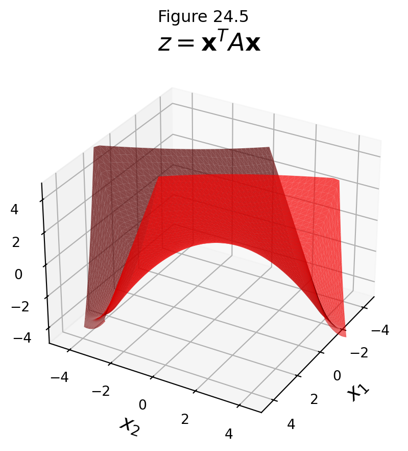
Clearly, we cannot minimize \(\mathbf{x}^TA\mathbf{x}\) over all \(\mathbf{x}\),
… but we can minimize \(\mathbf{x}^TB\mathbf{x}\) over all \(\mathbf{x}\).
How can we distinguish between these two cases in general?
That is, in high dimension, without the ability to visualize?
There is a remarkably simple way to determine, for any quadratic form, which class it falls into.
Theorem. Let \(A\) be an \(n\times n\) symmetric matrix.
Then a quadratic form \(\mathbf{x}^TA\mathbf{x}\) is
1. positive definite if and only if the eigenvalues of \(A\) are all positive.
2. positive semidefinite if and only if the eigenvalues of \(A\) are all nonnegative.
3. indefinite if and only if \(A\) has both positive and negative eigenvalues.
4. negative semidefinite if and only if the eigenvalues of \(A\) are all nonpositive.
5. negative definite if and only if the eigenvalues of \(A\) are all negative.
Proof.
A proof sketch for the positive definite case.
Let’s consider \(\mathbf{u}_i\), an eigenvector of \(A\). Then
\[\mathbf{u}_i^TA\mathbf{u}_i = \lambda_i\mathbf{u}_i^T\mathbf{u}_i.\]
If all eigenvalues are positive, then all such terms are positive.
Since \(A\) is symmetric, it is diagonalizable and so its eigenvectors span \(\mathbb{R}^n\).
So any \(\mathbf{x}\) can be expressed as a weighted sum of \(A\)’s eigenvectors.
Writing out the expansion of \(\mathbf{x}^TA\mathbf{x}\) in terms of \(A\)’s eigenvectors, we get only positive terms.
Example. Let’s look at the four quadratic forms above, along with their associated matrices:
\[A = \begin{bmatrix}3&0\\0&7\end{bmatrix}\]
\[A = \begin{bmatrix}3&0\\0&0\end{bmatrix}\]
\[A = \begin{bmatrix}2&0\\0&-1\end{bmatrix}\]
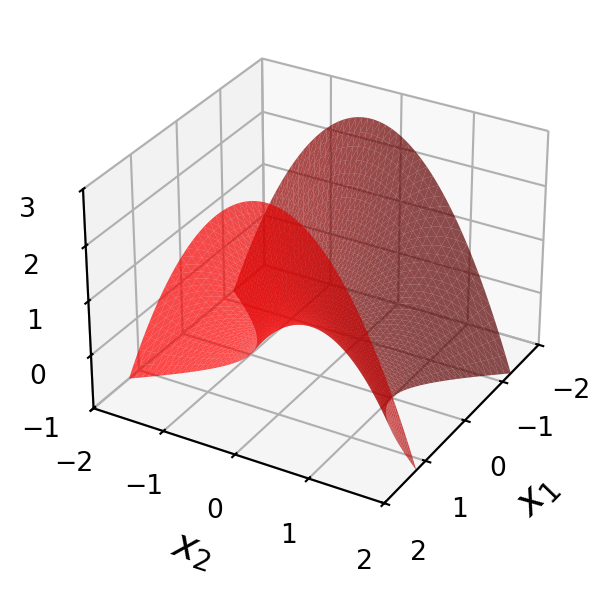
\[A = \begin{bmatrix}-3&0\\0&-7\end{bmatrix}\]
Example. Is \(Q(\mathbf{x}) = 3x_1^2 + 2x_2^2 + x_3^2 + 4x_1x_2 + 4x_2x_3\) positive definite?
Solution. Because of all the plus signs, this form “looks” positive definite. But the matrix of the form is
\[\begin{bmatrix}3&2&0\\2&2&2\\0&2&1\end{bmatrix}\]
and the eigenvalues of this matrix turn out to be 5, 2, and -1.
So \(Q\) is an indefinite quadratic form.
Constrained Optimization
A common kind of optimization is to find the maximum or the minimum value of a quadratic form \(Q(\mathbf{x})\) for \(\mathbf{x}\) in some specified set.
This is called constrained optimization.
For example, a common constraint is to limit \(\mathbf{x}\) to just the set of unit vectors.
While this can be a difficult problem in general, for quadratic forms it has a particularly elegant solution.
The requirement that a vector \(\mathbf{x}\) in \(\mathbb{R}^n\) be a unit vector can be stated in several equivalent ways:
\[\Vert\mathbf{x}\Vert = 1,\;\;\;\;\Vert\mathbf{x}\Vert^2=1,\;\;\;\;\mathbf{x}^T\mathbf{x} = 1.\]
Here is an example problem:
\[\text{minimize } 3x_1^2 + 7x_2^2 \text{ subject to } \Vert\mathbf{x}\Vert = 1 \]
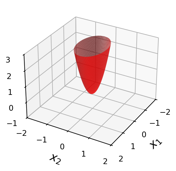
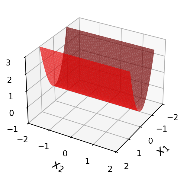
Let’s visualize this problem.
Here is the quadratic form \(z = 3x_1^2 + 7x_2^2\):
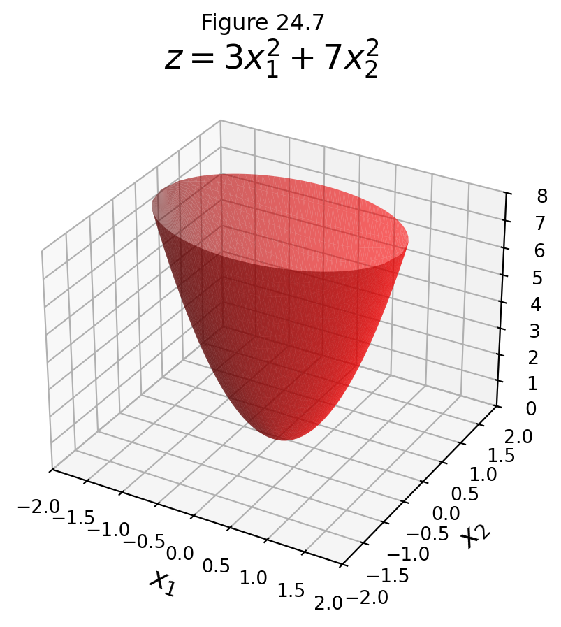
Now the set of all vectors \(\Vert\mathbf{x}\Vert = 1\) is a circle.
We plot this circle in the \((x_1, x_2)\) plane in green,
and we plot the value that \(z\) takes on for those points in blue.
Intersection of quadratic form \(z = 3 x_1^2 + 7 x_2^2\) and \(\Vert \mathbf{x}\Vert = 1\)
The set of blue points is the set \(z = 3x_1^2 + 7x_2^2\) such that \(\Vert \mathbf{x}\Vert = 1\).
Now, we can see the geometric sense of a constrained optimization problem.
In particular, we can visualize the solutions to two constrained optimizations:
\[ \min 3x_1^2 + 7x_2^2 \text{ such that } \Vert\mathbf{x}\Vert = 1 \]
and
\[ \max 3x_1^2 + 7x_2^2 \text{ such that } \Vert\mathbf{x}\Vert = 1 \]
Solving Constrained Optimization Over Quadratic Forms
When a quadratic form has no cross-product terms, it is easy to find the maximum and minimum of \(Q(\mathbf{x})\) for \(\mathbf{x}^T\mathbf{x} = 1.\)
Example. Find the maximum and minimum values of \(Q(\mathbf{x}) = 9x_1^2 + 4x_2^2 + 3x_3^2\) subject to the constraint \(\mathbf{x}^T\mathbf{x} = 1.\)
Since \(x_2^2\) and \(x_3^2\) are nonnegative, we know that
\[4x_2^2 \leq 9x_2^2\;\;\;\;\text{and}\;\;\;\;3x_3^2\leq 9x_3^2.\]
So
\[Q(\mathbf{x}) = 9x_1^2 + 4x_2^2 + 3x_3^2\]
\[\leq 9x_1^2 + 9x_2^2 + 9x_3^2\]
\[=9(x_1^2 + x_2^2 + x_3^2)\]
\[=9\]
Whenever \(x_1^2 + x_2^2 + x_3^2 = 1.\) So the maximum value of \(Q(\mathbf{x})\) cannot exceed 9 when \(\mathbf{x}\) is a unit vector.
Furthermore, \(Q(\mathbf{x}) = 9\) when \(\mathbf{x}=(1,0,0).\)
Thus 9 is the maximum value of \(Q(\mathbf{x})\) for \(\mathbf{x}^T\mathbf{x} = 1\).
A similar argument shows that the minimum value of \(Q(\mathbf{x})\) when \(\mathbf{x}^T\mathbf{x}=1\) is 3.
Eigenvalues Solve Contrained Optimization
Observation.
Note that the matrix of the quadratic form in the example is
\[A = \begin{bmatrix}9&0&0\\0&4&0\\0&0&3\end{bmatrix}\]
Proof: Since \(A\) is symmetric, it has an orthogonal diagonalization \(P^TAP = D = \operatorname{diag}(\lambda_1, \lambda_2, \dots, \lambda_n)\).
Since \(P\) is orthogonal, if \(\Vert\mathbf{x}\Vert = 1\), then \(\Vert P\mathbf{x}\Vert = 1\).
So, for any \(\mathbf{x}\), define \(\mathbf{y} = P\mathbf{x}\).
\[\max_{\mathbf{x}^T\mathbf{x} = 1} \mathbf{x}^TA\mathbf{x} = \max_{\mathbf{y}^T\mathbf{y} = 1} \mathbf{y}^TD\mathbf{y}\]
\[ = \max_{\mathbf{y}^T\mathbf{y} = 1} \sum_{i=1}^n \lambda_i y_i^2 \]
\[ \leq \max_{\mathbf{y}^T\mathbf{y} = 1} \lambda_1 \sum_{i=1}^n y_i^2 \]
\[ = \lambda_1.\]
Note that equality is obtained when \(\mathbf{x}\) is an eigenvector of unit norm associated with \(\lambda_1.\)
So the eigenvalues of \(A\) are \(9, 4,\) and \(3\).
We note that the greatest and least eigenvalues equal, respectively, the (constrained) maximum and minimum of \(Q(\mathbf{x})\).
In fact, this is true for any quadratic form.
Theorem. Let \(A\) be an \(n\times n\) symmetric matrix, and let
\[M = \max_{\mathbf{x}^T\mathbf{x} = 1} \mathbf{x}^TA\mathbf{x}.\]
Then \(M = \lambda_1\), the greatest eigenvalue of \(A\).
The value of \(Q(\mathbf{x})\) is \(\lambda_1\) when \(\mathbf{x}\) is the unit eigenvector corresponding to \(\lambda_1\).
A similar theorem holds for the constrained minimum of \(Q(\mathbf{x})\) and the least eigenvector \(\lambda_n\).